Adjustment of an integral function with Python

Python is a very convenient companion for function adjustment and scientific computing in general. We present in this article a simple problem where the scipy package is the sufficient toolbox to tackle an non linear adjustment problem involving a numerical integration.

Forewords

The scipy package is built on top of numpy which exposes the basis for linear algebra (multi dimensional arrays, products) and wraps specific linear algebra library including the famous LAPACK library.

The scipy package can be seen as a collection of numerical recipes to solve scientific daily life problems: integration, optimization, statistics, and so on…

This is the purpose of this article, showing through a simple numerical experience how this different topics can seamlessly be integrated together.

Debye model

Let’s say we want to assess Debye Temperature for Aluminium () and we have an experimental dataset of Internal Energy measurements w.r.t. Thermodynamic Temperature using the Debye model.

Then if we want to evaluate the Debye Temperature for Aluminium we must solve the following problem:

Where is the Debye function of order 3 defined as follow:

Adjusting such a function to experimental dataset is a Non Linear Least Squares problem (NLS for short) involving a numerical integration.

Problem statement

First we import required packages and for reproducibility sake we fix the random seed:

import numpy as np
from scipy import integrate, optimize, stats
import matplotlib.pyplot as plt
np.random.seed(123)

Then, we create a function factory for the Debye function:

def Debye(n):
    
    def integrand(t):
        return t**n/(np.exp(t) - 1)
    
    @np.vectorize
    def function(x):
        return (n/x**n)*integrate.quad(integrand, 0, x)[0]
    
    return function

This factory encompasses the Python magic, it solves a parametrized numerical integration problem in a vectorized way.

Finally, we instantiate the Debye function of order 3 using our factory and our objective function become as simple as:

D3 = Debye(3)

def energy(x, theta):
    return 3*x*D3(theta/x)

Where the theta parameter is the Debye Temperature we want to adjust from our experimental dataset.

Synthetic dataset

Lets create a synthetic experimental dataset to support the discussion. We create 20 points ranging from 25 to 550 K and evaluate energy for those temperatures. We add 10 units of absolute uncertainty on evaluated energy using a standard normal distribution.

TD = 428
T = np.arange(25, 551, 20)
Un = energy(T, TD)

Ur = Un + 10*np.random.randn(Un.size)

Adjustment

At this point everything is ready for fitting. We adjust the objective function to our synthetic dataset providing an initial guess of 300K:

parameters, covariance = optimize.curve_fit(energy, T, Ur, (300,))
# (array([424.20465445]), array([[11.97832334]]))

The adjusted temperature seems to be a fair estimate:

nsd = stats.norm()
z = nsd.ppf(0.975)               # 1.959963984540054
CI = z*np.sqrt(covariance[0,0])  # 6.783379383753078

We can evaluate the quality of the regressed parameter which is about for a 95% confidence interval which includes the theoretical value used to generate the dataset.

Finally, the figure below shows the adjusted energy curve:

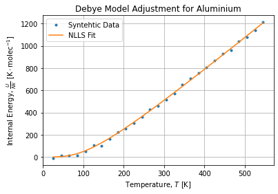
We can see frozen states effect when temperature is close to the absolute minimum and the quasi linear behavior when temperature is high above the Debye Temperature.

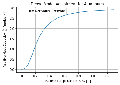
And the figure below shows the first derivative estimate w.r.t. Temperature of the adjusted curve. We indeed find the expected sigmoid curve from the Debye model:

Conclusions

We have shown through a specific example the capability of scipy package to solve a real scientific problem involving multiple knowledge areas such as integration, optimization and statistics.

We have shown using a synthetic dataset and a classic computer that computations are bearable and meaningful.

Finally we want to highlight some important concepts to keep in mind when adjusting model to data. Whenever we want to perform a numerical adjustment, key points are:

• Gather meaningful and consolidated dataset. We created a synthetic one for the occasion.
• Properly define the objective function to ensure numerical stability. We used a vectorized function factory and a specific integration method to model the objective function.
• Ensure convergence by providing both numerical stability and educated initial guess. We used a initial temperature in the range where Aluminum is solid.
• Criticize the adjustment result using optimization metadata and prior knowledge. We assessed a confidence interval for the regressed parameters and compared against the theoretical value.