Python and scipy package are very powerful when dealing with optimization problem. We present in this article a double optimization problem involving root find of a rational trigonometric equation and a non linear adjustment of a series expansion.
Modified Crank’s model
One dimensional partition by pure diffusion of a substrate between a liquid solution and a solid sphere can be modeled as follow:

A known series expansion solution to this problem has been developed by [Crank 1980] in the Mathematics of Diffusion.
The model can be adjusted to cope with the fact that substrate can have different affinities for liquid and solid phases considering the partition equilibrium is several magnitude order faster before diffusion characteristic time [Landercy 2011]. By considering the mass balance of the problem, the model can be expressed in term of liquid phase concentration instead of solid phase concentration. Those modifications leads to:

Where the  terms are solution of a rational trigonometric equation such as:

And the modified  coefficient equals to:

This model reformulation can be used to experimentally follow diffusion reaction of a substrate between liquid phase and solid spheres by measuring its concentration in the bulk of the liquid phase.
Problem statement
The goal is to regress partition  and diffusion
  coefficients from a function defined as an infinite series expansion involving the resolution of a rational trigonometric equation. An additional complexity is equation solutions are dependent of the coefficient therefore they need to be evaluated at each optimization step.
Solution presented in this article only require scipy package (which is built on top of numpy).
import numpy as np
from scipy import optimize
Root finding
First we need to solve the rational trigonometric equation. A bit of analysis shows that each positive root is contained in a well defined interval and is unique for each interval.
![q_n \in \left[\left(i -\frac{1}{2}\right)\pi, \left(i +\frac{1}{2}\right)\pi\right] \forall i \in \mathbb{N}_0](https://landercy.be/wp-content/ql-cache/quicklatex.com-8cd6f8c5f7e2bf0feecd868d7ba8b067_l3.png "Rendered by QuickLaTeX.com")
Figure below shows first positive roots for a typical value of .

Additionally, we recall that root finding problem defined as:

Can be translated into a minimization problem as follow:

Combining everything, we define a class to address this specific part of the problem. It implements the root finding strategy and produce the nth first solutions of the equation.
class EquationSolver:

    def __init__(self, alpha):
        self.alpha = alpha
        self.roots = {}

    def lhs(self, x):
        return np.tan(x)

    def rhs(self, x):
        return 3*x/(3 + self.alpha*x**2)

    def interval(self, n):
        return (-np.pi/2 + n*np.pi, np.pi/2 + n*np.pi)

    def objective(self, x):
        return (self.lhs(x) - self.rhs(x))**2

    def root(self, n):
        if n not in self.roots:
            result = optimize.minimize_scalar(
                self.objective,
                method="bounded",
                bounds=self.interval(n)
            )
            self.roots[n] = result.x
        return self.roots[n]

    def compute(self, n):
        solutions = []
        for i in range(n):
            solutions.append(self.root(i + 1))
        return np.array(solutions)
Curve fitting
Expansion limit
First, we must notice that the series term:

Is strictly positive and monotonically decreasing with respect to  and and it tends to zero as or tends to
  . Indeed this is a desirable property of the problem as we will need to limit the series expansion to a finite number of terms.
The figure below shows term magnitudes for typical values of partition and diffusion coefficients at different times when the series index  increases.
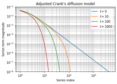
It highlights than precision issues are more important for early times, specially at the time  when the decreasing exponential is inhibited. This observation is confirmed when evaluating the associated series partial sum:
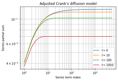
Except for early times, series partial sums converges quickly and taking a minimum of  terms seems sufficient at a first glance.
Implementation
We define a class to compute the series expansion and perform the coefficients regression.
class CrankDiffusion:

    def __init__(self, alpha=3, radius=1.9e-3, n=40):
        self.n = n
        self.alpha = alpha
        self.radius = radius
        self.objective = np.vectorize(self._objective, excluded='self')

    def alpha_prime(self, Kp):
        return self.alpha/Kp

    def solutions(self, Kp):
        return EquationSolver(self.alpha_prime(Kp)).compute(self.n)

    def term(self, t, qn, Kp, D):
        return np.exp(-(D*t*qn**2)/(self.radius**2))/(9*(self.alpha_prime(Kp) + 1) + (self.alpha_prime(Kp)**2)*qn**2)

    def sum(self, t, Kp, D):
        return np.sum([self.term(t, qn, Kp, D) for qn in self.solutions(Kp)])

    def _objective(self, t, Kp, D):
        return self.alpha_prime(Kp)/(1 + self.alpha_prime(Kp)) + 6*self.alpha_prime(Kp)*self.sum(t, Kp, D)
We initialize an object with the ad hoc experimental setup parameters and  :
:
S = CrankDiffusion(alpha=3, radius=1.9e-3)We load experimental dataset or generate synthetic dataset as follow:
texp = np.logspace(0, 6, 20)
rexp = S.objective(texp, 3.9, 2e-11) + np.random.randn(texp.size)*0.005
Adjustment
At this point everything is setup, we can perform the optimization as usual:
S = CrankDiffusion(alpha=3, radius=1.9e-3)
parameters, covariance = optimize.curve_fit(S.objective, texp, rexp, (5, 1e-10))
# (array([3.82165918e+00, 2.12262244e-11]),
# array([[ 1.56471526e-03, -2.22461680e-14],
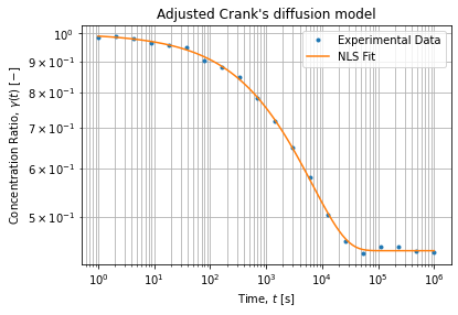
# [-2.22461680e-14, 5.97073552e-25]]))The figure below shows the adjusted model on a log-log scale:
Figures below show parameter variation and accuracy w.r.t. to the series expansion limits:
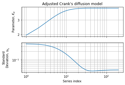
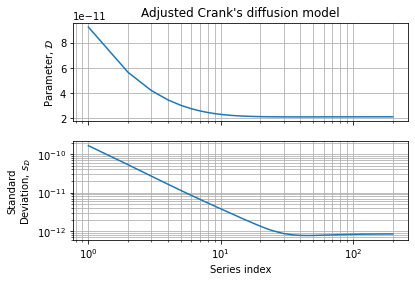
This numerical assessment shows than 40 terms is a good compromise between speed and accuracy. We also observe a region between 40 and 200 terms where accuracy seems bounce a bit. This behavior can be explained by an increase in variance when series becomes more complete w.r.t. experimental dataset. It should not be seen as an accuracy loss but rather as better convergence: the function we want to adjust needs an infinity of terms to converge to the exact function. If we can computationally afford more series terms we can increase the accuracy of the covariance matrix (and the confidence intervals we can draw from it) while the parameters estimation is no more improved.
Of course ad hoc expansion limit and observations are dependent on the experimental dataset and the expected values of the regressed parameters.
Figure below shows contours of the Parameters Optimization Surface (logarithm of Mean Squared Error) for the current dataset. Dashed lines stand for expected value of parameters, green point is our initial guess.
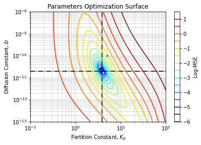
The surface strongly looks like a single minimum in a convex region within plausible range of parameters. It tends to confirm the adjustment converged toward the global optimum.
Conclusions
We have shown python and scipy can solve a nice problem involving root finding and series expansion adjustment. It is definitely a good companion to solve this applied physical chemistry problem.
We make use of class because it helps to produce cleaner code when solving complex problems. We also make use of numpy vetcorization to make function signature compliant with optimizers.
In addition of adjustment procedure, we added insights to highlight why and how it works mathematically and numerically. We have not covered everything in details but we think it is sufficient to get the big picture.
We hope this kind of snippet would be useful to researcher who needs to tackle equivalent scientific problems. Don’t hesitate to leave us a constructive feedback.
References
- [Crank 1980] J. Crank, The Mathematics of Diffusion, 2e Edition Oxford University Press, USA, 1980
- [Landercy 2011] J. Landercy, Contributions to removal of triclosan in wastewaters using enzymatic catalyst laccase immoblizated in porous Alg-PVA beads, ULB/UBT, 2011
