Multiple adjustments of a catalytic kinetic

Model

We want to model an heterogeneous reaction between Isopropanol and Raney’s Nickel which is a catalytic deshydrogenation. Reaction produces Isopropanone (acetone) and dihydrogen:

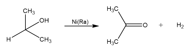
For sake of simplicity we label the reaction as follow:

$\mathrm{A \underset{Ni}{\overset{k_1}{\longrightarrow}} B + C}$

Where $k_1$ is the kinetic constant of the reaction which is governed by chimisorption of reactant and products on the catalyst surface. Using the isothermal model for monosorption the kinetic can be modelled follow:

$r = k_1 \theta_A = k_1\frac{aA}{1 + aA + bB + cC}$

By taking an ad hoc experimental setup (solution bulk is pure Isopropanone, hydrogen is continuously withdrawn from the system) we can simplify this model to:

$r = \frac{\mathrm{d}\xi}{\mathrm{d}t} \simeq k_1\frac{aA}{aA + bB} = k_1\frac{a(n_0 - \xi)}{a(n_0 - \xi) + b\xi}$

Where $\xi$ is the reaction coordinate and $a, b$ are reactant and product respective affinities for the catalyst surface. This ODE is separable:

$\int\limits_0^\xi\left(1 + \frac{b\xi}{a(n_0-\xi)}\right)\mathrm{d}\xi = \int\limits_0^t k_1\mathrm{d}t$

And leads to an explicit function for time w.r.t reaction coordinate:

$\left(1 - \frac{b}{a}\right)\xi - n_0\frac{b}{a}\ln\left|\frac{n_0 - \xi}{n_0}\right| = k_1t$

Based on this model we can assess two chemical constants by monitoring the reaction kinetic simply by logging produced hydrogen volume as a function of time.

Experimental dataset

We import some useful packages:

import numpy as np
import pandas as pd
import matplotlib.pyplot as plt

We define the experimental setup parameters and constants:

R = 8.31446261815324  # J/mol.K
T0 = 292.05           # K
p0 = 101600           # Pa
V = 190e-3            # L of Isopropanol
m = 2.7677            # g of Raney Nickel
rho = 785             # g/L
M = 60.1              # g/mol
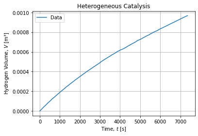
n0 = rho*V/M          # mol

Then we import an experimental dataset and compute some columns of interest:

df = pd.read_csv("data.csv")
df["xi"] = p0*df["V"]/(R*T0)
df["x1"] = df["xi"]/(n0 - df["xi"])
df["x2"] = np.log(np.abs((n0 - df["xi"])/n0))

The experimental raw time series looks like:

Notice we are presenting $\xi(t)$ relation in figures but adjustments will happen in the converse way $t(\xi)$ as we cannot create and explicit function for $\xi$ w.r.t. to time $t$ .

Ordinary Least Squares

First we must realize that adjusting the model function is an Ordinary Least Squares problem:

(1) $\begin{align*}t(\xi) &= \frac{1-k_2}{k_1} \xi + \left(-\frac{k_2}{k_1}n_0\right)\ln\left|\frac{n_0 - \xi}{n_0}\right| \\ &= c_1 x_1(\xi) + c_2 x_2(\xi)\end{align*}$

The variable $t$ it is linear combination of variables $x_1, x_2$ with weights $c_1, c_2$ .

This can be done with sklearn package as follow:

from sklearn.linear_model import LinearRegression

XOLS = df[["xi", "x2"]].values
yOLS = df["t"].values
OLS = LinearRegression(fit_intercept=False).fit(XOLS, yOLS)

OLS.score(XOLS, yOLS)  # 0.9999526276968934
OLS.coef_  # array([-1619.94014191,  1640.97679807])

The adjustment seems pretty good and graphically looks like:

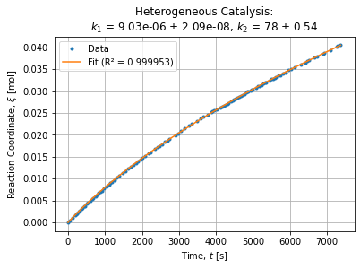
Then we can solve the system to express chemical constant w.r.t. OLS parameters:

$k_1 = \frac{n_0}{n_0c_1 + c_2} \,,\quad k_2 = \frac{-c_2}{n_0c_1 + c_2}$

Which equals to:

def solveOLS(c1, c2):
    k1 = n0/(n0*c1 + c2)
    k2 = -c2/(n0*c1 + c2)
    return k1, k2

k1OLS, k2OLS = solveOLS(*OLS.coef_)  # (9.03185366392649e-06, 78.00559108459133)

Generic fitting

We can also solve this problem in a more generic way using NLLS fit procedure as usual.

def factory(n0):
    def wrapped(x, k1, k2):
        return (1/k1) * ((1 - k2)*x - k2*n0*np.log((n0 - x)/n0)) 
    return wrapped

objective = factory(n0)
parameters, covariance = optimize.curve_fit(objective, df["xi"], df["t"])
# (array([9.03185361e-06, 7.80055898e+01]),
#  array([[4.38586891e-16, 1.11771567e-08],
#        [1.11771567e-08, 2.91368767e-01]]))

This result is identical to the OLS result but has the advantage to be straightforward and in addition provides an estimate of parameters covariance natively.

Lineweaver-Burk Linearization

In the early Nineteenth Century Ordinary Least Squares were already available. Anyway the method require a lot of computation which at the time had to be done by hand. Scientific also resorted to alternative method of determination in order to alleviate the computation load.

To solve such a problem, one can use the Lineweaver-Burk linearization method which consists to take the inverse of speed and express it w.r.t the ratio of Product/Reactant concentrations.

$r = k_1\frac{aA}{aA + bB} \rightarrow \frac{1}{r} = \frac{1}{k_1}\left(1 + k_2 \frac{\xi}{n_0 - \xi}\right)$

This method is easy to perform by hand because it is purely geometrical, it boils down to to regress a straight line though a point cloud and then assess its slope and intercept. But it requires to evaluates kinetic rates first.

First differences

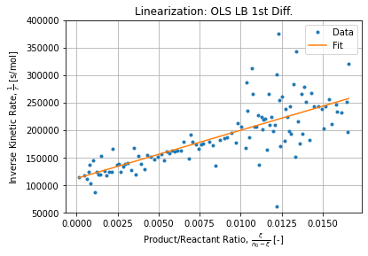
We can also estimates kinetic rates for each consecutive observation by evaluating the kinetic rates from the first difference ratio.

df["dxidt1"] = df["xi"].diff()/df["t"].diff()
df["1/r1"] = V/df["dxidt1"]

XLB = df[["x1"]].vakues[1:]
yLB = df["1/r1"].values[1:]

LB = LinearRegression(fit_intercept=True).fit(XLB, yLB)

LB.score(XLB, yLB)       # 0.565121006848629
k1LB = 1/LB.intercept_   # 8.933525882962039e-06
k2LB = LB.coef_[0]*k1LB  # 78.2451295539388

Figure below shows the regression:

Polynomial interpolation

One can try to interpolate the kinetic curve with a polynomial (of order 4 in this example) in order to assess kinetic rates from interpolated points.

from sklearn import preprocessing

XP3 = df[["t"]].values
yP3 = df["xi"].values

XP3f = preprocessing.PolynomialFeatures(degree=4).fit_transform(XP3)
P3 = LinearRegression(fit_intercept=True).fit(XP3f, yP3)
P3.score(XP3f, yP3)  # 0.9999768914232472

yP3hat = P3.predict(XP3f)

This is equivalent to develop the four first Taylor term for $t(\xi)$ . Then we can assess smoothed kinetic rates and perform the Lineweaver-Burk method again:

dCdt = np.diff(yP3hat)/df["t"].diff().values[1:]/V

XLBP3 = df[["xi"]].values[1:]
yLBP3 = 1/dCdt
LBP3 = LinearRegression(fit_intercept=True).fit(XLBP3, yLBP3)

LBP3.score(XLBP3, yLBP3)       # 0.9867005052472717
k1LBP3 = 1/LBP3.intercept_     # 8.801764527533865e-06
k2LBP3 = LBP3.coef_[0]*k1LBP3  # 73.22068510530787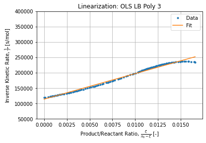

Observation are less dispersed in comparison with raw first difference but the series exhibits a structure (pattern of a rational function) which is directly linked to the polynomial adjustment we performed to estimate kinetic rates.

Method comparison

Figure below shows differences between methods used for assessing kinetic rates while performing the Lineweaver-Burk linearization.

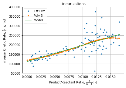
Each method has its advantages and drawbacks:

First differences method has a low correlation coefficient because of high points dispersion but the general direction is still plausible and does not requires any extra regression to evaluate kinetic rates which are defined as simple first difference ratios;
Polynomial interpolation has a good correlation coefficient but kinetic rates are not aligned. Instead they exhibit a wavely pattern due to its rational nature (inverse of polynomial).

Discussions

Table below shows for each method regressed coefficients including Correlation Coefficient and Chi Square Statistics as a goodness of fit metrics.

name	k₁	k₂	R²	Chi²
NLLS Integrated	9.0319e-06	78.006	0.99995	113.79
OLS Integrated	9.0319e-06	78.006	0.99995	113.79
OLS LB 1st Diff.	8.9335e-06	78.245	0.56512	1317
OLS LB Poly 3	8.8018e-06	73.221	0.9867	428.7

With no surprise OLS/NLLS has the minimal Chi Square as it is the metric it minimizes.

Figure below shows for each method the estimate of distribution of errors using Kernel Density Estimator for the OLS/NLLS adjsutment:

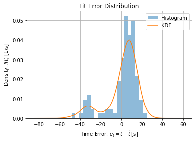
The error structure may point to a systematic error when operator change occurred in the middle of the experimentation. This change is visible as a break on the middle of the curve (see raw data). Restricting the dataset to observations before this change leads to a symmetric error structure:

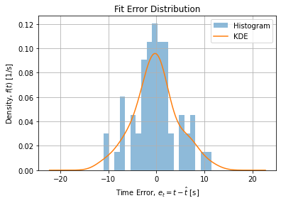
Figure below shows the Loss Function for the given dataset w.r.t. parameters over plausible range of values:

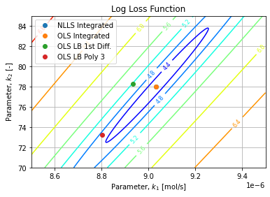
Regressed parameters in each method are reported over the surface contours. We observe the OLS/LMA methods converged to the Loss global minimum while other methods are their way around in the valley. Interestingly the LB First difference is closer to OLS method while having a bigger Loss than LB Polynomial.

The MSE surface exhibits a single minimum in a convex region which makes us confident the OLS/LMA converged to the global minimum.

Conclusions

This kinetic can be solved by OLS or NLLS with guarantee of optimality as the problem is linear in parameters. Lineweaver technique is useful, specially when OLS solver are not available (eg.: you are stuck in Excel) but it requires to estimate the kinetic rate which is not a trivial operation. First differences suffers from noise on data as derivation is an intrinsic unstable process. Fitting the kinetic with a polynomial is a bold approximation that introduces a bias while giving a comforting false impression of fitness. The problem is visible when taking the inverse of the rate which exhibits a rational curve behavior as expected.

Model

Experimental dataset

Ordinary Least Squares

Generic fitting

Lineweaver-Burk Linearization

First differences

Polynomial interpolation

Method comparison

Discussions

Conclusions

jlandercy

Related Posts

Find the closest points to a specific location using KD Tree

Compute Acid/Base Partition functions

Compute integral using Monte-Carlo