Using pollution roses to highlight traffic influence at Brussel’s 11th Canal Lock

Pollution rose is a very important tool when dealing with Air Quality Monitoring, they help to understand from which wind sectors the pollution arises and when correlating pollution roses at several locations it can be used to triangulate specific sources of pollution.

Wind

Wind speed

Wind speed is by nature a vector quantity. It has a major direct implication: there is no strict order to compare different wind speed measurements. It also implies than basic statistics don’t apply directly as they are defined for scalars.

A common approach to summarize wind speed measurements is to compute both vector $\bar{v}_v$ and scalar $\bar{v}_s$ arithmetic means:

$\bar{v}_v = \frac{1}{n} \left\lVert \sum\limits_{i=1}^n\mathbf{v}_i \right\rVert \, , \quad \bar{v}_s = \frac{1}{n}\sum\limits_{i=1}^n \left\lVert \mathbf{v}_i \right\rVert$

We must notice that in any case the following inequality holds:

$0 \leq \bar{v}_v \leq \bar{v}_s$

In addition of the quantity defined above the arithmetic mean of the vector phase (argument) – called mean wind direction $\bar{\theta}_v$ – is also computed. Of course this quantity is somehow meaningless as it an average of an angle unless vectors are stable in their direction within the aggregated sample.

Wind direction & stability

When wind direction is stable, vector and scalar mean speed are equals $\bar{v}_v = \bar{v}_s$ . When wind direction varies, vector mean speed is necessarily lower than scalar mean speed $\bar{v}_v \le \bar{v}_s$ . The edge case is a constant magnitude wind with isotropic direction (all sectors are equally probable over the aggregation period) which leads to a null vector mean speed $\bar{v}_v = 0$ while the scalar mean speed is positive $\bar{v}_s \ge 0$ . It implies the following ratio is constrained on the unitary segment:

$\gamma_k = \left(\frac{\bar{v}_v}{\bar{v}_s}\right)^k \in [0;1] \, \forall \, k \in \mathbb{N}_0$

A typical way to assess wind stability is to evaluate the following query $\gamma_7 \ge 0.95$ . Within aggregation period where the query holds we can both consider than the mean wind direction and the mean scalar speed are relevant and representative. In this case only we can reconstruct a mean vector representing the average wind during the aggregating period otherwise this average vector is pointless.

Wind speed distribution

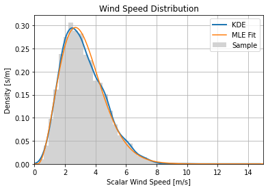
Wind speed is a positive definite quantity with a generally positively skewed distribution (left tail) often modeled as Weibull in literature. This means that mild winds are more likely than extreme wind. On the other hand extreme winds (gust) can have magnitude way above the mean wind speed (outliers).

Figure below shows a civil year of hourly scalar mean speed (41R001, 2014) with two density adjustments: KDE and Weibull MLE Fit.

Roses

Referential

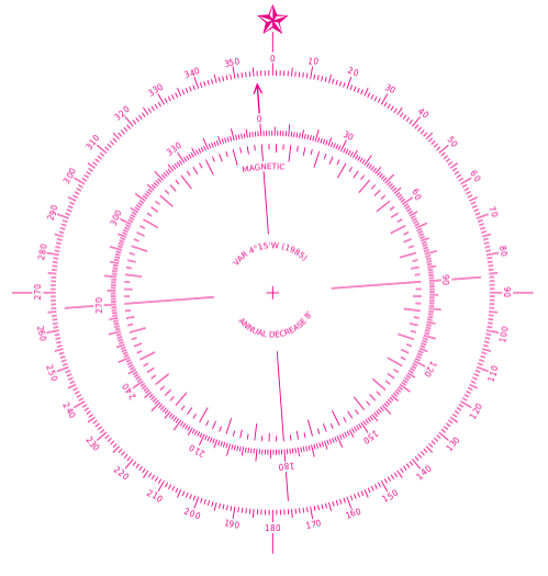
When dealing with wind speed measurements we must know in which referential angles are taken and in which direction wind is expressed. Wind vane generally publishes their wind directions in degrees (ranging from -90° to 450° to prevent jitter when passing by the North) in a goniometric referential (clockwise, origin located on North). This is very important to address this because it is not the same as the usual trigonometric referential (counter-clockwise, origin located on East).

Conversion formula (in radian) between goniometric angles $\theta_g$ and trigonometric angles $\theta_t$ is the following affine transformation:

$\theta_g = \frac{\pi}{4} - \theta_t$

It’s also important before drawing conclusion to know if the wind vane return direction of wind with respect to its origin or blowing from its origin. That is, wind vane measurements are vectors expressed as magnitude (wind speed) and angle (wind direction), but we also need to know the direction: Does the vector points towards origin or away from the origin?

Failing to address this aspect leads to mirrored and 90° shifted conclusions! A good way to assess this is to read the instrument operation manual and confront experimental measurements to common knowledge (eg.: prevailing winds).

Note: Depending of the application the direction of the rose may vary. Emission roses are generally pointing outwards origin as we want to plot where the matter goes, where immission roses are generally pointing towards origin as we want to plot where the matter comes from. In this article roses are immission roses.

Origin folding

Another problem we can face with wind direction measurements is the topology of the direction measurement space which is a one dimensional torus (circle) approximated by a linear scale. This leads to a strange behaviour at the ends of the direction scale: North can be approached either by 0° (coming from East) or 360° (coming from West). It means that if we have measurements coming from both directions an arithmetic mean of those directions will in fact be assumed as 180° South.

This is why wind vane generally publishes their directions over a range from -90° to 450°. When wind is coming from North, it forces angles to stay in a region where the average still is meaningful: providing an apparent continuity where the linear scale is broken.

Failing to address this specificity leads to misclassified wind directions and a classical symptom is an underpopulated North bin on wind and pollution roses. It is important to ensure the complete acquisition chain can handle this specificity (from the instruments to the data post-processing).

Imbalanced dataset

Because wind direction distributions are generally not isotropic dataset clustered on wind directions are not evenly distributed in term of observation count. Great care needs to be taken when comparing statistical quantities, aggregates and distributions. Don’t forget that more data means more chance to have outliers. Effect that is stronger in a world where concentrations distributions are positive definite and skewed.

Real situation

Prevailing winds

Figure below shows scalar mean speed distribution grouped by wind sectors:

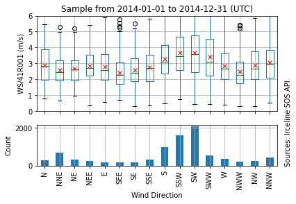
In Belgium, the prevailing winds are from the SW, but when the seasons change, the frequency of northeast winds is just as important. NE winds are polar, and therefore cold and dry.

The important information is wind sectors are imbalanced classes, wind direction is generally not isotropic in real dataset. The figure also shows slightly asymmetric distributions.

The figure complies with common knowledge, prevailing winds at this location comes from SW and SSW sectors (and the opposite directions NE and NNE) which is the natural orientation of Brussels riverbed. Thus, we can confirm with this figure above that data coming from this wind vane are expressed in goniometric angles with orientation towards the origin. Roses will read as follow, for each sector the aggregate is related to wind coming from this sector.

Figure below shows Brussels Digital Elevation Model (altitude scale) and map localization of the measuring site.

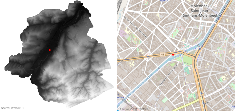
Brussels riverbed is the black strip (lowest altitudes) striking the DEM from SWW to NNE.

Figure below shows scalar wind speed measurement plotted over the wind rose grid (polar):

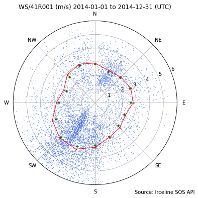
It highlights again the prevailing wind sectors and may indicate North class is underpopulated. Before going further we introduce a key concept to keep in mind when reading pollution roses: prevailing winds (more populated sectors) are not necessarily sectors with strongest measurements distributions. This is dependent of what are measured and how wind correlates with them. Indeed because they hold more observations they can exhibit stronger outliers.

Figure below shows a pollution rose with quantiles:

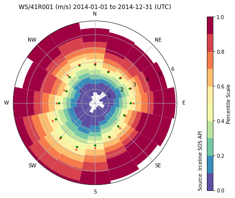
For this year, at this location prevailing winds were also strongest winds. Eg.: SW and SSW classes holds 20% of measurements above 5 m/s while other directions have less than 10% above this value. We also see mean (red cross) and median (green diamond) are shifted to higher wind speed values.

Traffic influence

Let’s see what happens when we correlate wind direction (read on the rose as “wind comes from this sector”) with chemical measurements. The site where the wind vane is located has a very peculiar urban context. It is located between the 11th lock along on the Brussel’s canal (at SW) and a high traffic avenue (Chaussée de Ninove, at NE). That makes this site somehow very convenient to analyze. To visualize this context, see the map above, the wind vane is located at the red dot.

Nitrogen Oxides

Let’s check first the Nitrogen Monoxide first as this substance is a good indicator (instable and reactive) for local combustion and thus for traffic and heating.

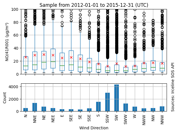
On this figure we can see that lower distributions arise on SW (more populated sectors at the canal side with more than 2000 observations) and higher distributions arise on NE (second most populated sectors at the avenue side with bins about 1000 observations). This where pollution rose becomes handy, the same dataset renders as follow:

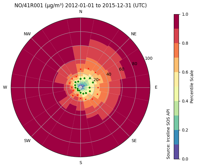
We can clearly spot on this figure the lower concentrations occurring at the canal side and higher concentrations coming from the avenue side.

If we check the Nitrogen Dioxide (more stable) which can transport on long distances the situation is totally different.

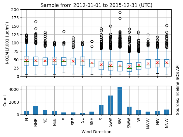
For Nitrogen Dioxide, distributions are less impacted by the wind direction. Because Nitrogen Oxide is also produced by combustion we still can see that SW sectors are in a smaller extent lower distributions but the effect is not as obvious as than Nitrogen Monoxide. Because Nitrogen Dioxide is more stable, it also can transport far away from it’s source, it is also normal that it’s concentration is more stable against wind direction.

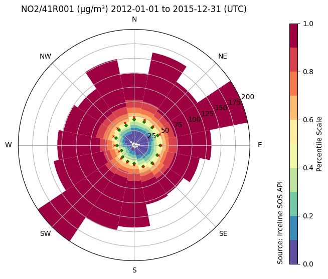
On this rose we see the combination of distant and local sources making the overall distribution more stable with respect to wind direction.

Black carbon

Black carbon is a granularity cut of soot absorbing light in visible spectrum and infra red region. There is no chemical standards for Black Carbon. Concentrations are sensor transduction defined by an arbitrary measurement methodology without chemical standards to calibrate on.

However, Black Carbon is known to strongly correlate with combustion involving carbonaceous substances such as traffic and heating. Additionally, Black Carbon is stable therefore it can transport on long distances, it is also removed from the atmosphere by dry and wet depositions.

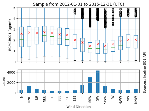
The trends around SW sectors is again visible on whisker boxes. The pollution rose renders it even better:

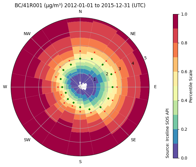
Distributions coming from avenue side are stronger than distributions coming from the canal side.

Conclusions

Pollution roses are a powerful tool to investigate Air Quality phenomena. For short, pollution rose correlates wind direction with chemical concentration allowing to plot on a single figure concentrations of pollutant and sectors it comes from or it goes by.

Single located rose can highlight local pollution source easily as we show with our “textbook case”. Confirmation of the source can be done by correlating multiple roses around the source and check if sector distributions geometrically converge.

Great care need to be taken when placing the wind vane over the field and caution during signal processing is required to get wind sector as accurate as possible. Failing to succeed my lead to erroneous conclusions in articles and models. A good thing to do is to check with common knowledge (reputed meteorological dataset) that at least prevailing winds are preserved after our computation.