Adjustment of an ordinary differential equation

This post shows how ODE parameters as well as initial condition can be adjusted to experimental data using Python. Adjusting ODE parameters is good topic to introduces specific methodology such as parameter normalization and sample bootstrapping.

Forewords

Disclaimer: I am not an epidemiologist. I will not draw epidemiological conclusions on parameters I will infer in this adjustment. The goal of this article is to show how we can fit ODE as well as other functions with Python. We chose the Belgium COVID Dataset to challenge fitting skills: the problem is know to be non trivial and include parameters normalization, bootstrapping and few other considerations. We chose this dataset because the nature of the model we want to apply and the dataset make the exercise very interesting if not trendy.

Model

There are several models involving ODE or system of ODEs to model epidemic dynamic. We choose here the adapted Generalized Richards Model (GRM for short) [Chowell 2017] which is a kind of modified logistic dynamic:

$\dot{C}(t) = \frac{\mathrm{d}C}{\mathrm{d}t} = r C^p\left[1-\left(\frac{C}{K}\right)^a\right]$

Where:

$C$ is the cumulative number of case (estimated from reported cases);
$r$ is the growth rate;
$p$ is the deceleration of growth (accounting for sub exponential peak);
$K$ is the size of the epidemic;
$a$ is the sigmoid deviation factor.

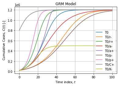
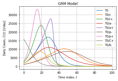
Typical GRM curves are flexible sigmoids:

Naive implementation

GRM can naively be modeled in Python as follow:

import numpy as np
import pandas as pd
from scipy import integrate, optimize

def GRM_ODE(t, C, r, p, K, a):
    return r*np.power(C, p)*(1-np.power((C/K), a))

def GRM(t, C0, r, p, K, a, rtol=1e-6):
    return integrate.solve_ivp(
         GRM_ODE, (t[0], t[-1]), [C0], t_eval=t,
         args=(r, p, K, a), rtol=rtol
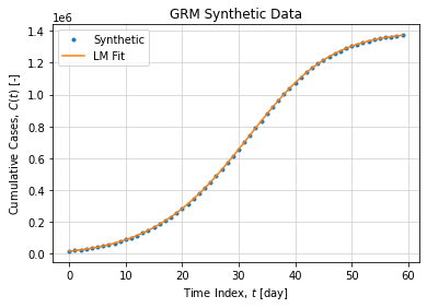
    ).y[0]

An adjustment with synthetic data without noise is shown below:

y = GRM(t, 1.7e4, 2.1, 0.76, 1.4e6, 2.1)

popt, pcov = optimize.curve_fit(
    GRM, t, y2, p0=(1e4, 1, 1, 1e6, 1),
    bounds=([1, 0.1, 0.01, 50, 0.1], [1e5, 10, 1, 1e7, 10]),
    gtol=1e-6, max_nfev=10000
)

# popt = [1.7e+04 2.1e+00 7.6e-01 1.4e+06 2.1e+00]
# pcov =
#               0             1             2             3             4
# 0  1.001441e-18 -3.695434e-22  1.431408e-23  8.930334e-19 -7.427668e-23
# 1 -3.695434e-22  1.602387e-25 -6.284162e-27 -5.550412e-22  3.730898e-26
# 2  1.431408e-23 -6.284162e-27  2.466777e-28  2.238019e-23 -1.479654e-27
# 3  8.930334e-19 -5.550412e-22  2.238019e-23  7.325558e-18 -1.967476e-22
# 4 -7.427668e-23  3.730898e-26 -1.479654e-27 -1.967476e-22  1.009053e-26

We are able to recover the initial parameters with a bit of configuration (tolerance, stop criterion, initial guess and parameters bounds). ODE are sensitive systems when handling them in computer sciences.

Graphically the adjustment looks like:

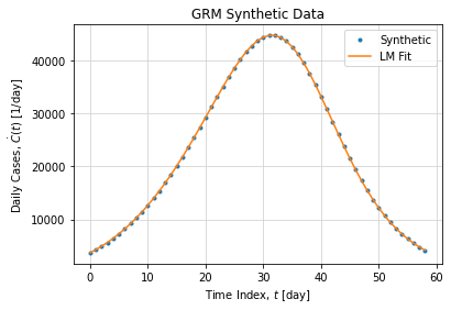
And leads to the following daily case peak:

The fact we can recover true parameter values in this synthetic example is not a guaranty of convergence. Solving ODE is not a trivial task, it is subject to numerical instabilities and initial condition variations. In addition we want to adjust parameters on top of a numerical ODE resolution, this add up a new layer of complexity. Finally, we must consider parameter scaling as C and K if not normalized are several magnitude order before other parameters.

Parameters normalization

Code below shows a handler class to solve this specific problem with parameters normalization:

class GRM:
    
    def __init__(self, scale=1e5):
        self.scale = scale
    
    def ode(self, t, C, r, p, K, a):
        return r*(np.power(C*self.scale, p)/self.scale)*(1-np.power(((C*self.scale)/(K*self.scale)), a))

    def objective(self, t, C0, r, p, K, a, rtol=1e-6):
        C0, r, p, K, a = self.scale_parameters(C0, r, p, K, a)
        solution = integrate.solve_ivp(
            self.ode, (t[0], t[-1]), [C0], t_eval=t, args=(r, p, K, a), rtol=rtol
        )
        return solution.y[0]*self.scale
    
    def scale_parameters(self, *p):
        p = np.array(p)
        p[0] /= self.scale
        p[3] /= self.scale
        return p
    
    def solve(self, t, C, sigma=None, p0=None, bounds=None, gtol=1e-9, max_nfev=25000):
                    
        if p0 is None:
            p0 = (1e4, 0.5, 0.5, 1e6, 0.5)
        
        if bounds is None:
            bounds = ((1, 1e-2, 1e-3, 1, 1e-2), (1e6, 5.0, 1, 9e9, 1e1))
       
        popt, pcov = optimize.curve_fit(
            self.objective,
            np.array(t), np.array(C), sigma=sigma,
            p0=p0, bounds=bounds, method="trf",
            gtol=gtol, max_nfev=max_nfev
        )
                
        return popt

This class can adjust the same ODE as previous but parameters $C$ and $K$ are down scaled by a factor $10^5$ to make them have the same magnitude order than others parameters.

Dataset

We targeted the Sciensano dataset which is the official source for Belgium COVID epidemic data.

data = pd.read_json("https://epistat.sciensano.be/Data/COVID19BE_CASES_AGESEX.json")
data["DATE"] = pd.to_datetime(data["DATE"])
tso = data.groupby("DATE")["CASES"].sum().to_frame()

Figures below show the full dataset and the last peak:

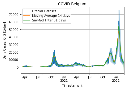
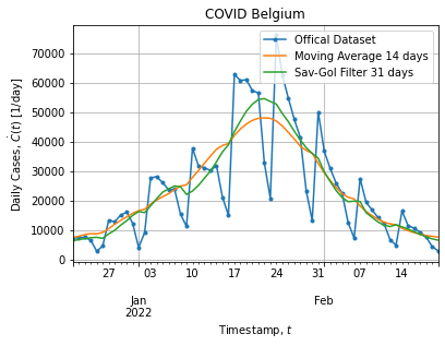
Of course the dataset is noisy as it is a real world data. In addition dataset exhibits a weekly structure: weekend cases are probably under-reported and cause downshoot on Saterday and overshoot on Monday, hence the weekly pattern.

Method

We will proceed as follow:

Download official data
Implement a normalized model for the GRM
Preprocess dataset:
- Smooth data with two techniques (moving average and sav-gol filter)
- Select a specific time range to isolate peak
- Resample at 6h resolution with linear interpolation (x4 w.r.t. daily data)
Bootstrap samples (n=200) and adjustment:
- Resample and then sample with replacement for 3 datasets :
  - Original data (Raw)
  - Moving Average (MV14D)
  - Savitsky-Golay filter (SG31D)
- Adjust normalized GRM parameters with Levenberg-Marquart algorithm while solving ODE using RK45 algorithm (adapting meta parameters)
Compare results

Preprocessing

We preprocess dataset in order to create new columns (smooth, first difference):

cases = data.groupby("DATE")["CASES"].sum().to_frame()
cases["index"] = (cases.index - cases.index[0])//pd.Timedelta("1d")
cases["cumsum"] = cases["CASES"].cumsum()
cases = cases.reset_index().rename(columns={"CASES": "daily", "DATE": "date"}).set_index("date")
cases["cs_mv14d"] = cases["cumsum"].rolling(14).mean().shift(-7)
cases["d_mv14d"] = cases["cs_mv14d"].diff()
cases["cs_savgol"] = signal.savgol_filter(cases["cumsum"], 31, 7)
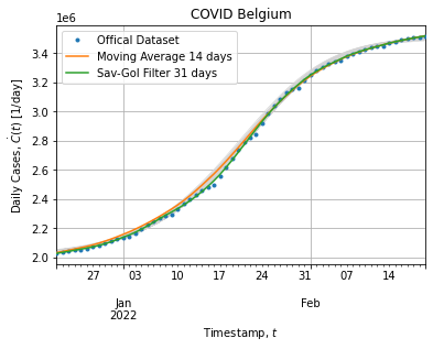
cases["d_savgol"] = cases["cs_savgol"].diff()

Figure below shows the dataset subject to the adjustment:

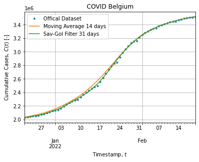
The Savitzky-Golay filter (31 days, 7th order) stick to cumulative cases and smooth out weekly down-shoot while the Moving Average (14 days) take off a bit when the peak rises.

Bootstrap

The following code resample dataset (increase observations by a factor 4) and sample at random with replacement in order to have sufficient observations for bootstrapping:

def resample(frame):
    sample = frame.copy()
    # Reindex:
    sample = frame.set_index("index_origin")
    index = np.arange(sample.index.min(), sample.index.max() + 0.001, 0.25)
    sample = sample.reindex(index).interpolate().reset_index()
    # Resample:
    sample = sample.sample(frac=1.0, replace=True).sort_index()
    # Deduplicate + Counts:
    count = sample.groupby(sample.index)["index"].count()
    count.name = "count"
    sample = sample.drop_duplicates().merge(count, left_index=True, right_index=True)
    sample = sample.sort_index()
    sample["sigma"] = np.sqrt(1/sample["count"])
    return sample

Notice we introduced and adapted sigma to cope with duplicate sample. Then each bootstrap sample is adjusted:

params = []
for i in range(200):
    # Resampling:
    sample = resample(peak)
    print(i, sample.shape[0])
    # Adjusting:
    popt, pcov = optimize.curve_fit(
        GRM,
        sample["index_origin"].values, sample["cumsum_origin"].values/scale, sigma=sample["sigma"].values,
        p0=(2.2e4/scale, 1.0, 0.75, 1.5e6/scale, 2.1),
        bounds=([1/scale, 1e-2, 1e-2, 50/scale, 0.1], [1e5/scale, 10, 1, 1e7/scale, 10]),
        gtol=1e-9, max_nfev=25000
    )
    params.append(popt)
params = pd.DataFrame(params, columns=["C", "r", "p", "K", "a"])

The procedure is repeated for each dataset (Raw, MV14D and SG31D).

Results

We chose to present here the result for the SG31D because we found it was the better compromise between parameters RSD and MSE w.r.t. raw data. Same observations can be drawn for Raw and MV14D adjustments.

Figure below shows bootstrap adjustment for daily cases (what have been derived from adjusted curve):

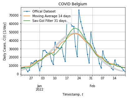
Figure below shows bootstrap adjustment for cumulative cases (what actually have been adjusted):

Each bootstrap adjustment exhibits the same behavior: curves remains above the cumulative distribution when peak rises and then saturates when peak falls back. It might suggest that our model does not fit well the peak extracted from the dataset. This is not surprising it is not a single peak epidemic.

Table below show the bootstrap parameter statistics:

	C	r	p	K	a
count	200	200	200	200	200
mean	17951.709434	2.109440	0.763941	1.491274e+06	2.129987
std	1801.121558	0.534494	0.020363	4.192278e+03	0.131553
min	13676.831795	1.028284	0.700643	1.470937e+06	1.796077
25%	16817.081914	1.711702	0.751492	1.488802e+06	2.042899
50%	17629.907849	2.071898	0.763188	1.491130e+06	2.133465
75%	18997.914543	2.375822	0.779201	1.493932e+06	2.219590
max	25707.487672	4.440710	0.820486	1.502641e+06	2.582613

Figures below show the bootstrap parameter distributions:

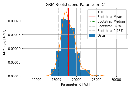
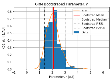
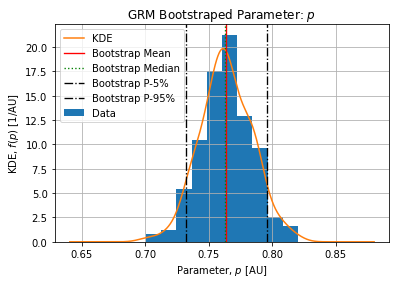
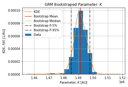
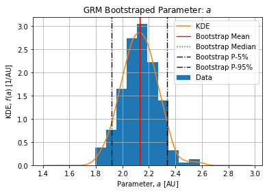
Table below shows the Relative Standard Deviation of each parameters:

	Raw	MV14D	SG31D
C	0.109941	0.104995	0.100331
r	0.290582	0.183442	0.253382
p	0.030304	0.021949	0.026655
K	0.002975	0.002246	0.002811
a	0.065908	0.045842	0.061763

Bootstrapping parameters is showing CLT in action: the standardized parameters distribution are most likely normal distributions:

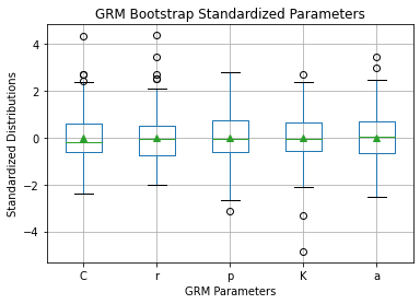
With a confidence threshold of 10% we could not reject this hypothesis of Kolmogorov-Smirnov test H0: standardized parameters are sampled from standard normal distribution. Table below shows the KS statistic and the p-value of the KS test.

Parameter	Location	Scale	KS Statistic	p-value
C	1.296740e-15	0.997497	0.080350	0.143109
r	8.659740e-17	0.997497	0.065699	0.338981
p	-1.110223e-15	0.997497	0.039186	0.906524
K	2.784439e-15	0.997497	0.047484	0.739512
a	-5.817569e-16	0.997497	0.030478	0.989722

Conclusions

How satisfied are you with the fit?

Compared to the other fits presented in previous post, the selected model does not fit with the same goodness the selected peak extracted from dataset. Let’s criticize it.

We must consider that the model might not match properly the dataset because it has extra structures in it (weekly pattern) and the selected peak will not validate all model hypothesis. It is not an isolated single-waved peak with stable condition during it time frame. Instead it is the third peak of an almost 2 years running epidemic happening just before the end of the year when social and cultural events are likely to happen.

GRM models is a simple logistic like model for a single wave, in this adjustment we see it does not fit perfectly smoothed data as well. GRM fits raise and fall quicker than smoothed data. GRM model also expects the cumulative count to saturate to $K$ (daily case tends to 0) when time increases, which is not certain.

A very touchy part in addition of having a regressed curve that does not stick perfectly to the dataset is the strong variation of solution an ODE can have when its parameters or its initial condition vary slightly. This makes ODE adjustment more sensitive than adjustments in previous posts.

Off course there can have some methodological or implementation errors we haven’t caught yet. Please don’t hesitate to raise it in a comment, we will be glad to address it.

This said, the adjusted model does capture a general picture of the peak and this is somehow satisfying even if we know that it might not be the better model to describe this dataset.

How satisfied I am with this adjustment? Not satisfied enough to say the GRM is eligible to model the dataset accurately. But it does not mean it we cannot say anything about the adjustment and the procedure itself.

How would you criticize adjusted parameters?

This post also illustrated the bootstrapping technique which puts the Central Limit Theorem in action and allow us to assess the variability of adjusted parameters. We confirmed parameter distributions are likely to be normal. Further more, introducing bootstrapping in the process highlighted the need for parameters normalization. Once done we reduced the RSD of this parameter $r$ from 0.8 to 0.25 which is an improvement for such a sensitive parameter.

Even if the model is not satisfactory in describing the exact shape of the peak, adjusted parameters are not totally meaningless. We present here a 5% confidence interval for each parameters without claiming any epidemiological sense of those values:

The epidemic size $K = (1.4913 \pm 0.0082)\times 10^6$ is coherent with the number of detected cases on the selected dataset. On the selected peak 1486374 cases arose from 2021-12-21 to 2022-02-20. The complete epidemic size is slightly above which is expected.

The deceleration of growth $p = 0.764 \pm 0.040$ is sub-exponential meaning the beginning of the peak (when logistic term is close to unity) grows slower than an exponential.

The growth rate $r = 2.1 \pm 1.0$ is the parameter with the higher uncertainty and its meaning is directly linked w.r.t. the deceleration of growth factor $p$ . It globally controls the strength of the peak.

The sigmoid deviation factor $a = 2.13 \pm 0.26$ is moderate and makes the solution a bit asymmetrical with a peak fall happening quicker than the peak raise.