We present in this article a quick but complete overview of the GDAL powerful capabilities using a trivial example: assessing the GPS altimeter dataset compared with respect to Brussels’ Offical Digital Elevation Model. Goals are two: showing by examples how GDAL can ease professional GIS integration into Database and having fun while exploiting a personal dataset to check if the altimeter of my GPS helps in elevation estimation.
Make sure GDAL environment is properly setup
We will need a fonctinnal GDAL setup for this one, you may skip this section if your GDAL/PostGIS setup already is working in terminal.
When we deal with GIS we generally have multiple versions of GDAL installed (specially on Windows) as each GIS product (PostGIS, GQIS, OSGeo4W, and so on) comes with its own version (just in case it was not enough messy). Often GDAL commands break because this binding is incomplete or mixed. GDAL setup relies on three essential environment variables:
- GDAL_DATA which contains all GDAL configurations;
- GDAL_DRIVER_PATH which contains all source drivers (including PostgreSQL driver);
- PROJ_LIB which contains projection database GDAL needs to performs its operations.
In this example we decide to rely on GDAL from QGIS installation as we know the software is able to perform all GIS operations with PostgreSQL seamlessly, meaning the GDAL version of QGIS is aligned with our PostgreSQL+PostGIS database setup.
SET GDAL_DATA=C:\Program Files\QGIS 3.16.15\share\gdal
SET GDAL_DRIVER_PATH=C:\Program Files\QGIS 3.16.15\bin\gdalplugins
SET PROJ_LIB=C:\Program Files\QGIS 3.16.15\share\proj
In addition the exact PATH variable sequence is of importance as it will determine which GDAL commands will be executed. Ensure GDAL from QGIS comes before PostgreSQL binaries as it also pack GDAL if you installed PostGIS.
echo %PATH%
...;C:\Program Files\QGIS 3.16.15\bin;C:\Program Files\PostgreSQL\14\bin;...
If the setup is mixed and GDAL versions are different we are in trouble and we will need to align version prior to unleash the GDAL power. Classical symptoms are error complaining about projection versions or database driver.
Additionally, if it’s not done yet, we will play with both vector and raster data, so we need both PostGIS extension to deal with those kind of data. Ensure your PostgreSQL database has installed the following extensions:
CREATE EXTENSION postgis;
CREATE EXTENSION postgis_raster;
Building datasets
Digital Elevation Model
First we will import the official Brussels’ DEM from UrbIS OpenData portal. Original raster file is a TIF file of a resolution of 1mx1m over the Brussels’ Region area with a single band for the elevation, the file size is about 2.8 Gb. First we will reduce the resolution to 5mx5m pixels that will be enough wrt. GPS precision (100Mb):
gdalwarp -tr 5 5 -r cubicspline brussels/dem_1m.tif brussels/dem_5m.tif

Creating output file that is 3800P x 3800L.
Processing brussels/dem_1m.tif [1/1] : 0Using internal nodata values (e.g. 0) for image brussels/dem_1m.tif.
Copying nodata values from source brussels/dem_1m.tif to destination brussels/dem_5m.tif.
...10...20...30...40...50...60...70...80...90...100 - done.
Then we tile the file into square of 25mx25m before inserting it into a raster layer in our PostgreSQL database. Tiling is important as it allows us to build and index to drastically fasten GIS queries.
raster2pgsql -s 31370 -c -F -C -I -t 25x25 brussels/dem_5m.tif references.dem_brussels | psql -p 5432 -d mygis -U jlandercy
INSERT 0 1
...
INSERT 0 1
CREATE INDEX
ANALYZE
NOTICE: Adding SRID constraint
NOTICE: Adding scale-X constraint
NOTICE: Adding scale-Y constraint
NOTICE: Adding blocksize-X constraint
NOTICE: Adding blocksize-Y constraint
NOTICE: Adding alignment constraint
NOTICE: Adding number of bands constraint
NOTICE: Adding pixel type constraint
NOTICE: Adding nodata value constraint
NOTICE: Adding out-of-database constraint
NOTICE: Adding maximum extent constraint
addrasterconstraints
----------------------
t
(1 row)
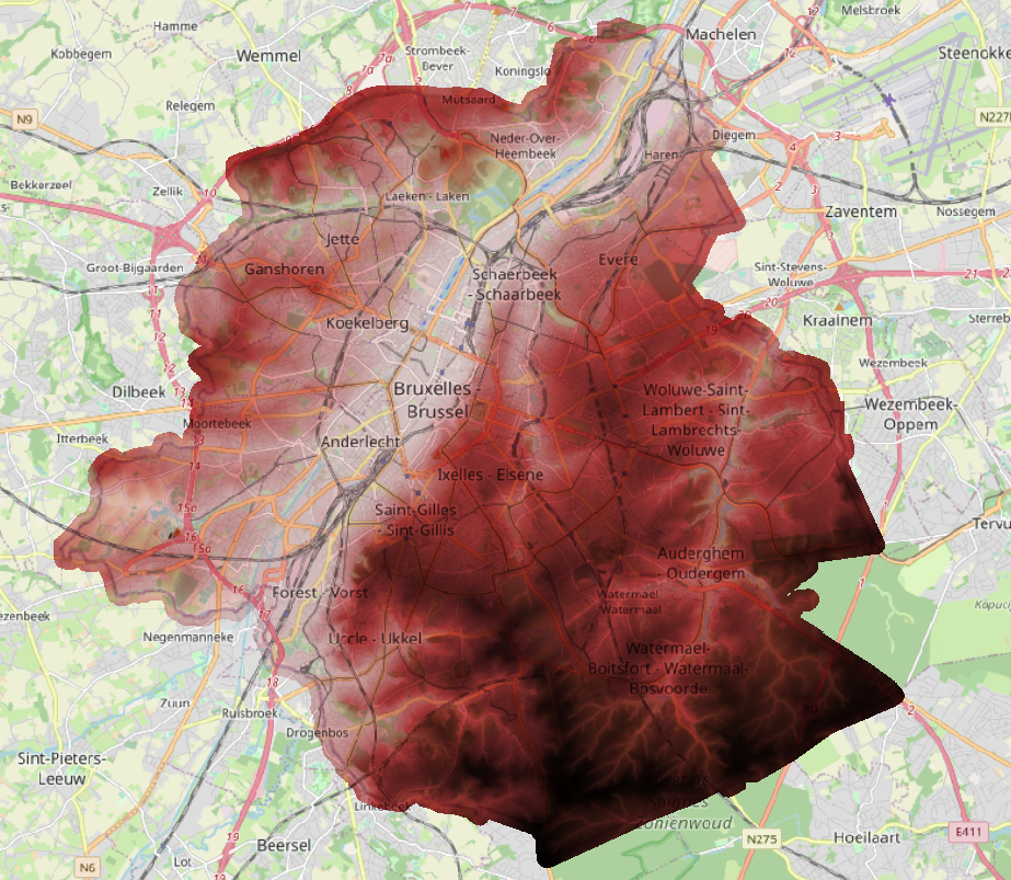
COMMITNow the DEM can be loaded quickly and efficiently as a raster layer into QGIS:
Elevation contours
Meanwhile we are processing the DEM, it costs nothing to create elevation contours.
gdal_contour -a elev -i 1.0 dem_5m.tif contours.shp

0...10...20...30...40...50...60...70...80...90...100 - done.
Which produces a Shape File with elevation contours that can be imported using GDAL as well:
shp2pgsql -c -S -I -s 31370 brussels/contours.shp references.brussels_contours | psql -U jlandercy -h localhost -p 5432 -d mygis

Field elev is an FTDouble with width 24 and precision 15
Shapefile type: Arc
Postgis type: LINESTRING[2]
SET
SET
BEGIN
INSERT 0 1
...
INSERT 0 1
CREATE INDEX
COMMIT
ANALYZE
Final results by level of 10m looks like:
SELECT *
FROM "references"."dem_brussels_contours"
WHERE elev::INTEGER % 10 = 0;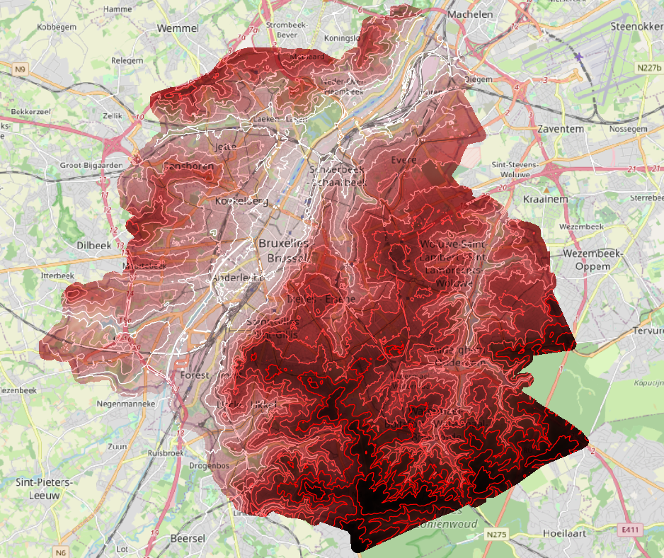
GPS dataset
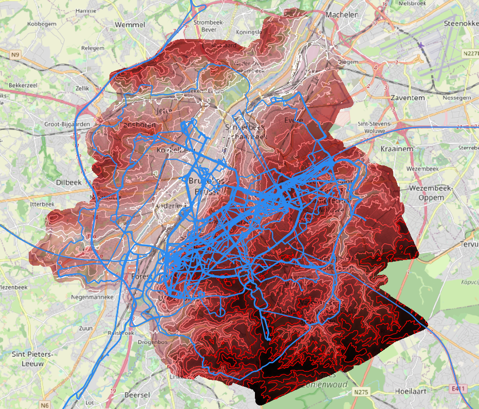
Time to import some GPS tracks of interest: here a collection of bike trips in Brussels mixed with some other stuffs that we will filter out before we can perform our analysis. We have exported our dataset into the GPX format from the GPS management interface and we insert it into our database:
ogr2ogr -f PostgreSQL "PG:host=localhost port=5432 dbname=mygis user=jlandercy password=secret-token" -lco SCHEMA=jlandercy tracks.gpxIt creates five tables in specified schema. Raw dataset looks like (tracks):
Now we needs to filter out points of interests and convert it into correct SRID on the raster bounding box and reindex geometries into this new SRID to perform quick and efficient queries.
DROP MATERIALIZED VIEW IF EXISTS jlandercy.brussels_points;
CREATE MATERIALIZED VIEW jlandercy.brussels_points AS
WITH

-- Select DEM bounding box:
RC AS (
SELECT *, ST_Transform(extent, 4326) AS bbox
FROM public.raster_columns
WHERE r_table_name = 'dem_brussels'
)

-- Select points within this bounding box:
SELECT
	P.*,
	ST_Transform(
		wkb_geometry, 31370
	)::Geometry(Point, 31370) AS geom   -- This casting is necessary for PostGIS registry
FROM
    jlandercy.track_points AS P JOIN RC
		ON ST_Contains(RC.bbox, wkb_geometry)
;

-- Index new geometry with DEM compatible SRID to speed up computation:
CREATE INDEX jlandercy_brussels_points_index
ON jlandercy.brussels_points USING gist(geom);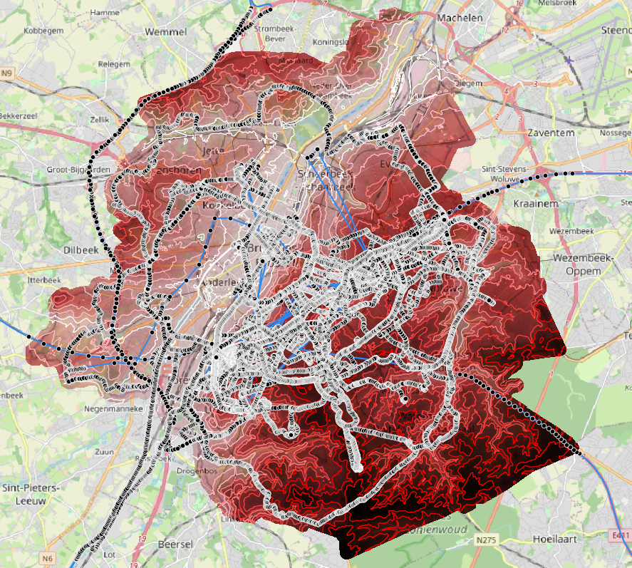
Mapping DEM elevation to points
Now we will map DEM elevation to each GPS points and compare the DEM official value with GPS recorded elevation.
DROP MATERIALIZED VIEW IF EXISTS jlandercy.brussels_elevation;
CREATE MATERIALIZED VIEW jlandercy.brussels_elevation AS
WITH
data AS (
SELECT
P.*,
ST_Value(D.rast, P.geom) AS ele_ref,
D.rid
FROM
jlandercy.brussels_points AS P JOIN "references".dem_brussels AS D
ON ST_Intersects(D.rast, geom)
)
SELECT
*,
(ele - ele_ref) AS abs_error,
(ele - ele_ref)/ele_ref AS rel_error,
ABS((ele - ele_ref)/ele_ref) AS abs_rel_error
FROM data
WHERE ele_ref IS NOT NULL;
CREATE INDEX jlandercy_brussels_elevation_index
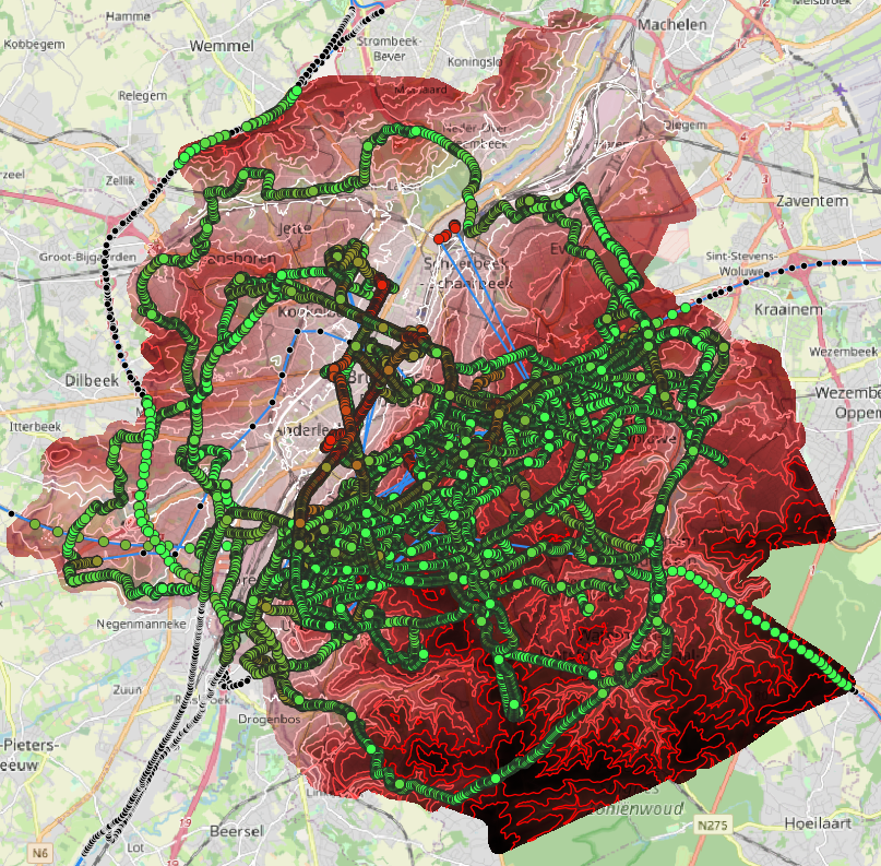
ON jlandercy.brussels_elevation USING gist(geom);The figure below show absolute value of relative error for selected points. Green points have less than 50% of error which is still high. We will take it into account in next section.
Analyzing GPS/DEM dataset
Raw dataset
Now we have a complete dataset to analyze where we have mapped on GPS points expected elevation extracted from DEM. Table below summarizes dataset:
| GPS Elevation [m] | DEM Elevation [M] | Absolute Error [m] | Relative Error [-] | Track Time [min] | |
|---|---|---|---|---|---|
| count | 116848.000000 | 116848.000000 | 116848.000000 | 116848.000000 | 116848.000000 |
| mean | 63.469261 | 65.145625 | -1.676364 | -0.041538 | 973.302685 |
| std | 39.508907 | 22.941046 | 31.956043 | 0.595669 | 838.557097 |
| min | -818.680000 | 7.587822 | -899.664808 | -11.574002 | 0.000000 |
| 25% | 43.690000 | 48.000172 | -10.385776 | -0.161599 | 364.283333 |
| 50% | 66.100000 | 71.123385 | -3.376928 | -0.050744 | 585.816667 |
| 75% | 82.030000 | 81.482640 | 4.800151 | 0.080271 | 1471.033333 |
| max | 444.780000 | 126.937267 | 405.259249 | 10.254341 | 3486.233333 |
Prepared dataset contains about 110k points for which we successfully mapped DEM Elevation. We observe that GPS Elevation contains some obvious outliers at both side of the distribution: way deep in the see and way over Brussels highest point (about 110m). Dataset also contains a lot of long running tracks which will probably add some challenge for the data analysis as atmospheric pressure can vary a lot on hourly basis and GPS elevation is the result of a proprietary algorithm blending GPS fix and Altimeter measurements (actually a pressure sensor).
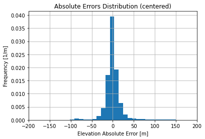
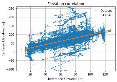
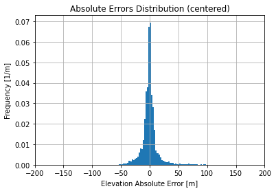
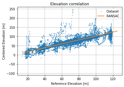
As a baseline, we show Absolute Errors and Elevation Correlation of the raw dataset:
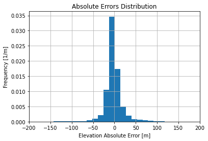
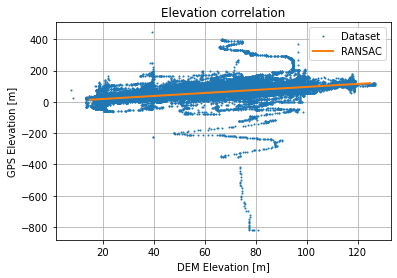
Absolute Errors distribution is not too skewed and looks like it is sharper than a normal distribution. Using a robust linear regression (RANSAC) we get the following regression  with a score about 0.343 which is not too bad given the thickness of the point cloud.
Smoothing the edges
This dataset suffers from two major flaws:
- Altimeter has not been calibrated before each use so the device algorithm needed several GPS fixes before calibrating wrt to GPS estimated elevation (which is the most imprecision axis for such a standard) and start to records relevant elevation points. This effect can be mitigated by removing first and last points of tracks when GPS is not yet calibrated and/or manipulated;
- Some tracks are recorded over long periods (more than several hours), for such tracks elevation drift is observed due to atmospheric pressure variation which participate as a signification elevation bias in both directions. Centering recorded elevation to have the same mean than reference can reduce the bias impact on the regression by minimizing the cloud thickness;
If we filter out first and last points and compare centered elevation instead of recorded elevation we can highlight the second flaw:
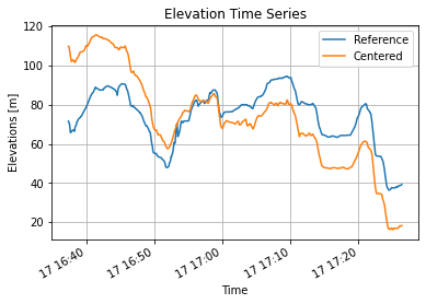
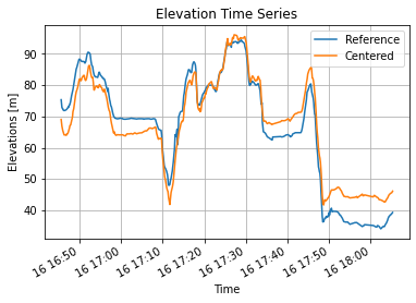
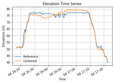
On the first track the atmospheric pressure was going heavier leading to a negative elevation drift (we are placed lower than expected), on the second track the atmospheric pressure was going lighter leading to a positive elevation drift (we are place higher than expected). When atmospheric pressure is stable, the correlation is almost perfect:
Challenging the dataset for regression we still have 111712 points and the regression is quite similar to the previous  with a score about 0.432. Graphically it renders as follow:
If we drastically filter out long tracks, keeping at most 10% of the dataset (about 13800 points) things become cleaner:
The regression becomes better with a slope which is still about the unity  with a score about 0.746 (cloud point thickness has reduced a lot).
Conclusions
We shown how to use GDAL commands to ingest and prepare layers into a GIS database in order to perform usual GIS queries.
Using prepared layers, we built a new dataset by mapping DEM elevation to GPS points allowing us to assess if the GPS elevation using the altimeter is relevant.
During the analysis, we performed three regression each having a slope close to unity and an offset relatively small before elevation range (few meters vs 10 kilometers).
Filtering problematic tracks indeed improved the correlation score which can be thought visually as a reduction of the point cloud thickness.
