Simultaneously adjust multiple kinetics

In this post we show how we can fit simultaneously multiple kinetics from ODE system using the scipy package. That is, we will regress parameters from multiples curves described by a dynamic system at once. To reach that goal, we will bind the optimization and integration capacities of scipy by defining function with ad hoc signatures, feed them properly and assess the result.

For this post, the following package are required:

import numpy as np
import numdifftools as nd
import matplotlib.pyplot as plt
from scipy import integrate, optimize, stats
from sklearn.metrics import r2_score

Defining the system

Lets say we want to model sequential reactions such as:

(1)  

With the following governing kinetics:

(2)  

In python we formulate the system as follow:

def system(t, x, k0, k1):
    return np.array([
        - k0 * x[0],
        + k0 * x[0] - k1 * x[1],
                    + k1 * x[1]
    ])

Solving the IVP

We want to solve the Initial Value Problem (IVP) for this ODE system. To perform this task we need to integrate the ODE system over a time range t, with some initial condition y0, for some constants that will be provided as args. On the other hand we want the solver method to be fitted by a minimizer so it must expose parameters as its first argument. Following function fulfill those constraints:

def solver(parameters, t=np.linspace(0, 1, 10)):
    solution = integrate.solve_ivp(
        system, [t.min(), t.max()], y0=parameters[-3:],
        args=parameters[:-3], t_eval=t
    )
    return solution.y

As stated, in order to be fittable, the solver method must have a specific signature with all parameters as the first variable (extra parameters comes after). In this implementation, the parameters vector contains first kinetics constants, then initial concentrations such as [k0, k1, x00, x10, x20].

At this point we can generate some synthetic dataset (texp, xexp, sigma) using the solver method to challenge our ODE solving procedure.

np.random.seed(12345)
p0 = np.array([ 0.85, 0.15, 1.5, 0.25, 0.])
texp = np.linspace(0, 10, 30)
xexp = solver(p0, t=texp)
sigma = 0.01 * np.ones_like(xexp) 
xexp += sigma * np.random.normal(size=xexp.shape)

Solving the NLLS Problem

Now we want to solve a Non Linear Least Squares (NLLS) problem. Usually we would use the handy curve_fit method, but it is limited to one dimensional function and we are facing a multidimensional function (solver returns 3 concentrations). Therefore we will have to formulate the Least Square problem by ourselves and minimize it.

We write the expression of a Chi Square loss function in term of our dataset and regressor:

def loss_factory(t, x, sigma):
    def wrapped(parameters):
        return 0.5 * np.sum(np.power((x - solver(parameters, t=t)) / sigma, 2))
    return wrapped

This function is a wrapper that will prepare ad hoc function to feed the minimizer. We create the loss function for the given dataset:

loss = loss_factory(texp, xexp, sigma)

Then performing the minimization is as simple as:

solution = optimize.minimize(
    loss,
    x0=[1, 1, 1, 1, 1],
    bounds=[(0, np.inf)] * 5
)
#       fun: 41.60636573541066
#  hess_inv: <5x5 LbfgsInvHessProduct with dtype=float64>
#       jac: array([-0.00301767, -0.01338876,  0.01562341,  0.01689315,  0.00656257])
#   message: 'CONVERGENCE: REL_REDUCTION_OF_F_<=_FACTR*EPSMCH'
#      nfev: 186
#       nit: 27
#      njev: 31
#    status: 0
#   success: True
#         x: array([0.8364894 , 0.15044452, 1.5001996 , 0.24623917, 0.00241979])

We can see that all parameters are close to their original values, recalling we have added normal noise of sigma = 0.01 mol/L on each concentration.

Notice we have added bound constraints on minimization in order to force the solver to stay in the positive real region for each parameter.

The figure below shows the adjustment for each concentration:

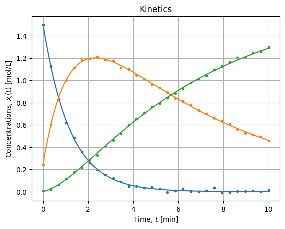
The result is visually satisfying, it seems the procedure did regress parameters properly. Now we should assess the quality of the solution.

Quality of the solution

Coefficient of determination

First we compute the coefficient of determination, we predict concentrations for regressed parameters and compare them to observed dataset:

xhat = solver(solution.x, t=texp)
score = r2_score(xexp, xhat)  # 0.999498540097489

Three nines is a nice global performance and it confirms the visual fitness on the figure above.

Goodness of Fit

We can also assess the Goodness of Fit (GoF) criterion by comparing the Chi Square statistics to its expected distribution:

chi2 = 2. * solution.fun  # 83.21273147082132
nu = xexp.size - p0.size  # 85
chi2n = chi2 / nu         # 0.9789733114214274

law  = stats.chi2(df=nu)
pvalue = law.sf(chi2)     # 0.5345849047291789

Normalized Chi Square is close to unity and the p-value of the GoF test is high. As a reminder, p-value is defined as:

In null-hypothesis significance testing, the p-value is the probability of obtaining test results at least as extreme as the result actually observed, under the assumption that the null hypothesis is correct.

Wikipedia

This comfort us in accepting the null hypothesis : each observation of the model are independent and normally distributed observation. Meaning we are confident in the fact that observed deviation from the model can be totally explained by the variance and are not due to the choice of the model itself or the nature of error distributions.

Parameter uncertainties

Finally we can evaluate the Hessian of the loss function at the solution in order to estimate the Covariance matrix .

H = nd.Hessian(loss)(solution.x)
C = np.linalg.inv(H)
np.sqrt(np.diag(C))
# [0.00583539, 0.00059994, 0.00595627, 0.00643674, 0.00338883]

Which return equivalent C matrix as the method curve_fit does. We have in addition of parameters, uncertainty estimations, therefore we do know how many significant digits we have got on each parameters. In this case: which both contains original parameters at .

Conclusions

We showed it is possible to simultaneously fit multiple kinetics. The strategy is simple, define the ODE system, create an ODE solver with signature compliant with the minimizer and minimize it against datasets.

Then, we also showed some post processing steps to assess the quality of the found solution: coefficient of determination, goodness of fit test, parameters covariance estimation.