Adjustments of a statistical distribution

This post shows how to adjust statistical distribution on a random sampled dataset and assess precision of regressed parameters.

Synthetic dataset

We create a synthetic dataset by sampling random values from a Log Normal law:

import numpy as np
import matplotlib.pyplot as plt
from scipy import stats, optimize
import numdifftools as nd
from sklearn.metrics import r2_score

np.random.seed(12345)
law = stats.lognorm(s=0.5, loc=0., scale=3.2)
N = 30000
data = law.rvs(size=N)
xlin = np.linspace(data.min(), data.max(), 200)
yth = law.pdf(xlin)

We also create a support for the random variable in order to estimate Probability Density Functions.

Native MLE

Module stats from scipy package can natively fit a distribution from random samples:

sol1 = stats.lognorm.fit(data, loc=0.)
# (0.4996375201174542, -0.0054040502417716995, 3.1993268382049647)

In this case it returns a tuple of three parameters (s, loc, scale), as the native MLE procedure fits all available parameters from the distribution.

yhat1 = stats.lognorm.pdf(xlin, *sol1)
score1 = r2_score(yth, yhat1)
# 0.9999872246793303

This method is very convenient as it directly returns parameters without the need of defining anything. On the other hand, we don’t have much information to say on regressed parameters.

Manual MLE

We can always write explicitly the MLE problem and minimize it by ourselves:

def likelihood_factory(x):
    def wrapped(p):
        return - np.sum(stats.lognorm.logpdf(x, s=p[0], loc=0., scale=p[1]))
    return wrapped

likelihood = likelihood_factory(data)

sol2 = optimize.minimize(likelihood, x0=[1, 1], method="Powell")
# message: Optimization terminated successfully.
# success: True
#  status: 0
#     fun: 56640.833635064184
#       x: [ 5.006e-01  3.193e+00]
#     nit: 4
#   direc: [[-8.934e-02 -7.337e-01]
#           [-3.010e-02  5.371e-02]]
#    nfev: 110

It returns fairly good values for parameters with the Powell method.

yhat2 = stats.lognorm.pdf(xlin, s=sol2.x[0], scale=sol2.x[1])
score2 = r2_score(yth, yhat2)
# 0.9999826981445005

The advantage of having the likelihood function explicitly defined wrt parameters is that we can estimate parameters covariance matrix from the Hessian:

H = nd.Hessian(likelihood)(sol2.x)
C = np.linalg.inv(H)
# array([[ 4.17608735e-06, -3.00263399e-09],
#        [-3.00263399e-09,  8.51575800e-05]])

We can also sketch the likelihood landscape wrt to parameters:

@np.vectorize
def loss(s0, s1):
    return likelihood([s0, s1])

s0 = np.linspace(0.1, 2.0, 100)
s1 = np.linspace(1, 10, 100)
S0, S1 = np.meshgrid(s0, s1)

L = loss(S0, S1)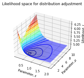

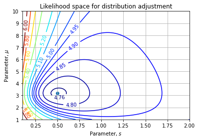
Then we can estimate the uncertainty on our parameters:

sp = np.sqrt(np.diag(C))
# array([0.00204355, 0.00922809])

Our regressed parameters are then (at one sigma interval).

Histogram adjustment

Another technique, which can be used when we don’t have the actual underlying data but only their distribution as an histogram. In this case, we directly curve_fit the PDF function to the histogram data.

def model(x, sigma, mu):
    return stats.lognorm.pdf(x, s=sigma, loc=0., scale=mu)

density, bins = np.histogram(data, bins=30, density=1.)
centers = (bins[:-1] + bins[1:]) / 2.

sol3 = optimize.curve_fit(model, centers, density)
# (array([0.51053274, 3.21758681]),
#  array([[5.00065660e-06, 3.75746621e-06],
#         [3.75746621e-06, 7.33786763e-05]]))

It’s important to have representative bins (enough observation in each bins). It also force us to chose a representative value for x, we chose bin center in this case.

yhat3 = model(xlin, *sol3[0])
score3 = r2_score(yth, yhat3)
# 0.999539309318677

If this method is less accurate than previous because of the data aggregation due to histogram, it has the advantage also returns the covariance estimate.

Methods comparison

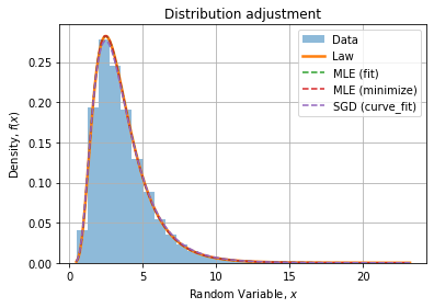
Visually, fits seem to agree with the data distribution and the theoretical PDF, with a slight deviation for the histogram fit (curve_fit) visible at the top of the peak.

We can compare absolute and relative errors wrt theoretical PDF:

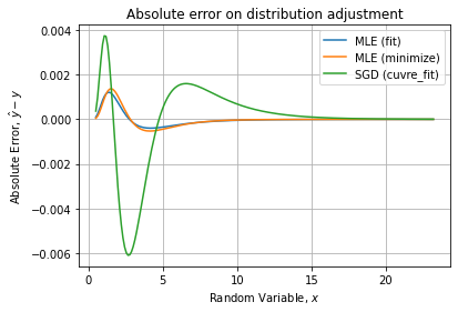
We see the depletion of the peak for the histogram fit.

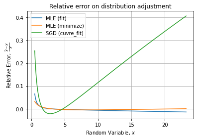
Checking for the relative error, it confirms the last method is the less accurate. Comparing only the two first gives:

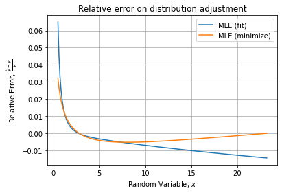
Indicating the manual MLE has the best relative error curve with less than 3% of error on the curve.