This post shows of to fit an arbitrary number of Lorentzian peaks (Cauchy distribution) using scipy.
import inspect
import itertools
import numpy as np
import matplotlib.pyplot as plt
from scipy import stats, signal, optimize
from sklearn.metrics import r2_score
Model
The key to be able to plot an arbitrary number of peaks is to design model signature properly. First we define the peak model as we usually does when using curve_fit.
def peak(x, x0, s, A):
    return - A * stats.cauchy(loc=x0, scale=s).pdf(x)
Then construct a multiple peak model with a single vector of parameters that must be a multiple of peak parameters:
def model(x, *p):
    m = len(inspect.signature(peak).parameters) - 1
    n = len(p) // m
    y = np.zeros_like(x)
    for i in range(n):
        y += peak(x, *p[i*m:(i+1)*m])
    return y
Indeed this function will not fit for curve_fit as it expect explicit parameters, but minimize will do.
Dataset
Lets construct a synthetic dataset with 6 peaks:
x0s = [10, 25, 70, 100, 120, 140]
s0s = [1, 1.5, 2, 1, 0.5, 1]
A0s = [2, 3, 2, 3, 1, 1]
p0 = list(itertools.chain(*zip(x0s, s0s, A0s)))
# [10, 1, 2, 25, 1.5, 3, 70, 2, 2, 100, 1, 3, 120, 0.5, 1, 140, 1, 1]
np.random.seed(123456)
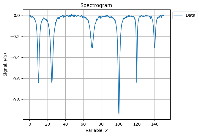
xlin = np.linspace(0, 150, 500)
y = model(xlin, *p0)
s = 0.005 * np.ones_like(xlin)
yn = y + s * np.random.normal(size=s.size)Which renders as:
Peak identifications
Now we need to automatically identify how many peaks we have and where they are located.
peaks, bases = signal.find_peaks(-yn, prominence=0.2)
# (array([ 33,  83, 233, 333, 399, 466]),
#  {'prominences': array([0.63486587, 0.61350699, 0.30987885, 0.94338495, 0.63369006,
#          0.30995799]),
#   'left_bases': array([  4,  51, 156, 156, 369, 434]),
#   'right_bases': array([156, 156, 287, 497, 497, 497])})
Peaks have been properly identified but base boundaries are a bit messy, we can clean them up:
def clean_base_indices(lefts, rights):
_lefts = np.copy(lefts)
_rights = np.copy(rights)
for i in range(len(lefts) - 1):
if lefts[i + 1] < lefts[i]:
_lefts[i + 1] = rights[i]
if rights[i + 1] < rights[i]:
_rights[i] = lefts[i + 1]
if lefts[i] == lefts[i + 1]:
_lefts[i + 1] = rights[i]
if rights[i] == rights[i + 1]:
_rights[i] = lefts[i + 1]
return _lefts, _rights
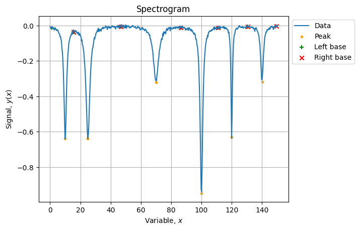
lefts, rights = clean_base_indices(bases["left_bases"], bases["right_bases"])
# (array([ 4, 51, 156, 287, 369, 434]), array([ 51, 156, 287, 369, 434, 497]))The result of identification looks like:
Fit parametrization
Using the peak identification data, we create initial conditions vector and bounds to help to drive the minimization:
x0 = list(itertools.chain(*[[xlin[i], 0.1, 0.1] for i in peaks]))
bounds = list(itertools.chain(*[
    [(xlin[lefts[i]], xlin[rights[i]]), (0., np.inf), (0., np.inf)] for i in range(len(peaks))
]))
We state the loss function (normalized Chi Square):
def loss_factory(x, y, s):
    def wrapped(p):
        return np.sum(np.power((y - model(x, *p)) / s, 2)) / (x.size - len(p))
    return wrapped

loss = loss_factory(xlin, yn, s)
And we perform its minimization helped by our educated initial guess and boundaries:
sol = optimize.minimize(loss, x0=x0, bounds=bounds)
# fun: 1.0955753119538643
# hess_inv: <18x18 LbfgsInvHessProduct with dtype=float64>
# jac: array([-2.73114841e-06, -4.70734565e-05, 6.31272816e-05, 1.57429612e-05,
# 3.73034939e-06, -2.41806576e-05, 1.29674131e-05, -5.59552408e-06,
# -2.22932785e-05, 1.63980044e-04, -1.13486998e-04, -5.48450177e-06,
# 6.19504837e-05, 6.61692919e-05, -3.19744233e-06, 2.42916605e-05,
# -2.20268249e-05, 1.53876912e-05])
# message: 'CONVERGENCE: REL_REDUCTION_OF_F_<=_FACTR*EPSMCH'
# nfev: 836
# nit: 41
# njev: 44
# status: 0
# success: True
# x: array([ 10.00233549, 1.01832565, 2.02107376, 24.99880996,
# 1.50914703, 3.01233404, 69.98152044, 2.04653551,
# 2.01075276, 99.98876123, 1.00539617, 3.00563652,
# 119.99496644, 0.50185139, 1.00415731, 140.00815263,
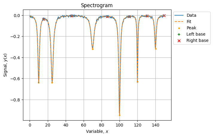
# 1.02170953, 1.00824265])Which is a fairly good optimization:
yhat = model(xlin, *sol.x)
score = r2_score(yn, yhat)  # 0.9986663779143068
The final result looks like: