Animated double pendulum

This post shows how to create an animated double pendulum with scipy and matplotlib.

Setup

First we import dependencies:

import numpy as np
from scipy import integrate
import matplotlib.pyplot as plt
from matplotlib.animation import FuncAnimation 

We define the physical constants of our problem:

L1 = 0.25
L2 = 0.20
L = L1 + L2
m1 = 1
m2 = 2
g = 9.81

We define the double pendulum model:

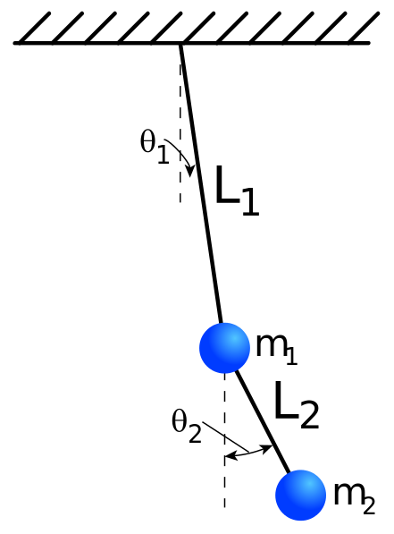
Where the system can be defined as:

   

   

Where:

   

This highly non linear system can be represented as follow:

def model(t, y, L1, L2, m1, m2, g):
    a1, a2, a1t, a2t = y
    da = a1 -a2
    M = m1 + m2
    alpha = m1 + m2 * np.sin(da) ** 2
    return np.array([
        a1t,
        a2t,
        (- np.sin(da) * (m2 * L1 * a1t ** 2 * np.cos(da) + m2 * L2 * a2t ** 2) - g * (M * np.sin(a1) - m2 * np.sin(a2) * np.cos(da))) / (L1 * alpha),
        (+ np.sin(da) * (M * L1 * a1t ** 2 + m2 * L2 * a2t ** 2 * np.cos(da)) + g * (M * np.sin(a1) * np.cos(da) - M * np.sin(a2))) / (L2 * alpha)
    ])

Solution

We integrate the system for a given set of initial conditions and our physical setup:

t = np.linspace(0, 25, 10000)
s = integrate.solve_ivp(
    model, [t.min(), t.max()],
    [np.pi/2, np.pi/2, 0, 0], t_eval=t,
    args=(L1, L2, m1, m2, g)
)
#   message: The solver successfully reached the end of the integration interval.
#   success: True
#    status: 0
#         t: [ 0.000e+00  2.500e-03 ...  2.500e+01  2.500e+01]
#         y: [[ 1.571e+00  1.571e+00 ...  2.601e-01  2.453e-01]
#             [ 1.571e+00  1.571e+00 ...  2.738e+01  2.740e+01]
#             [ 0.000e+00 -9.811e-02 ... -5.950e+00 -5.910e+00]
#             [ 0.000e+00 -3.260e-09 ...  9.336e+00  9.163e+00]]
#       sol: None
#  t_events: None
#  y_events: None
#      nfev: 4502
#      njev: 0
#       nlu: 0

Time solution looks like:

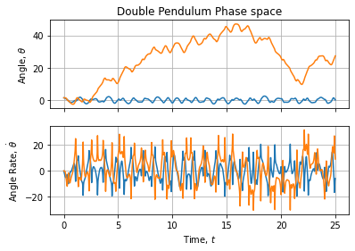
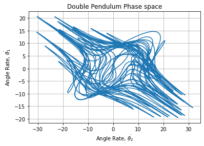
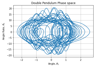
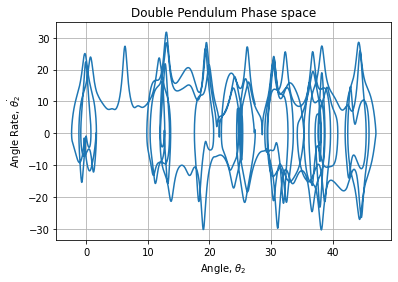
Phase spaces are about:

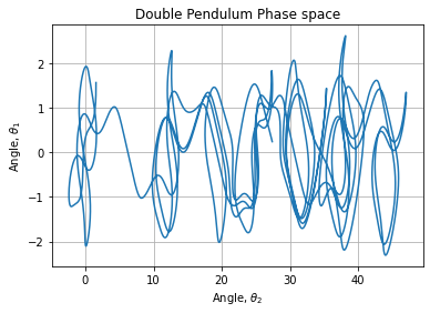
We transform radial coordinates into Cartesian coordinates:

def coordinate(s, L1, L2):
    x1 = L1 * np.sin(s.y[0, :])
    y1 = - L1 * np.cos(s.y[0, :])
    return np.array([
        x1,
        y1,
        x1 + L2 * np.sin(s.y[1, :]),
        y1 - L2 * np.cos(s.y[1, :])
    ])

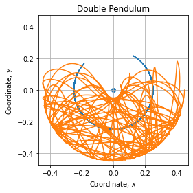
c = coordinate(s, L1, L2)

We check our pendulum is kept between its physical boundaries:

assert np.all(np.sqrt(c[2, :] ** 2 + c[3, :] ** 2) <= L)

Trajectory is about:

Animation

Now it’s time to create a nice animation:

fig, axe = plt.subplots()
text = axe.text(0., L * 0.9, "", horizontalalignment="center")
pendulum, = axe.plot([], [], "-o")
trajectory, = axe.plot([], [])

def init():
    axe.set_title("Double Pendulum")
    axe.set_xlabel("")
    axe.set_ylabel("")
    axe.set_xlim([-L*1.05, +L*1.05])
    axe.set_ylim([-L*1.05, +L*1.05])
    axe.set_aspect("equal")
    axe.grid()
    return pendulum, trajectory

def update(frame):
    text.set_text("t = %.3f [s]" % frame)
    q = ((frame - 2.) < t) & (t <= frame)
    i = np.where(q)[0].max()
    pendulum.set_data([0, c[0, i], c[2, i]], [0, c[1, i], c[3, i]])
    trajectory.set_data(c[2, q], c[3, q])
    return trajectory, pendulum

fps = 24
dt = t.max() - t.min()
n = int(fps * dt)

animation = FuncAnimation(fig, update, frames=np.linspace(t.min(), t.max(), n), init_func=init, blit=True)

animation.save(filename="AnimatedPendulum.gif", writer="pillow", fps=fps)

Which renders: