This post shows how to solve the Ballistic problem with Drag Force taken into account.
Setup
We import required libraries:
import numpy as np
import matplotlib.pyplot as plt
from scipy import integrate
The model can be expressed as follow:
![\[\bar{F} = m \bar{a} - c \bar{v}\]](https://landercy.be/wp-content/ql-cache/quicklatex.com-b59236aded82131d1203f23fa2982cdd_l3.png "Rendered by QuickLaTeX.com")
Which can be projected:
![\[\frac{\mathrm{d}^2x}{\mathrm{d}t^2} = - \frac{c}{m}v_x\,,\quad \frac{\mathrm{d}^2y}{\mathrm{d}t^2} = -g -\frac{c}{m}v_y\]](https://landercy.be/wp-content/ql-cache/quicklatex.com-25158612deab5f8bf783c8fca01fc5d6_l3.png "Rendered by QuickLaTeX.com")
And then linearized:
def model(t, x, m, g, c):
    return np.array([
        x[2],
        x[3],
        - c * x[2] / m,
        - g - c * x[3] / m
    ])
We also define two events function (root finding) for to trigger when Apex and Ground are found over the trajectory:
def apex(t, x, m, g, c):
    return x[3]
We monkey-patch the second function to interrupt the integration process when projectile hit the ground:
def ground(t, x, m, g, c):
    return x[1]
ground.terminal = True
ground.direction = -1
Solution
We integrate the system:
sol = integrate.solve_ivp(
    model, [0., 10.], [0., 0.50, 50., 10.],
    events=(apex, ground), args=(0.25, 9.81, 1.),
    dense_output=True
)
We refine the time grid based on the solution found:
t = np.linspace(sol.t.min(), sol.t.max(), 200)
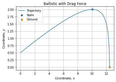
x = sol.sol(t)We plot the refined solution and event coordinates:
fig, axe = plt.subplots()
axe.plot(x[0,:], x[1,:], label="Trajectory")
axe.scatter(sol.y_events[0][0, 0], sol.y_events[0][0, 1], label="Apex")
axe.scatter(sol.y_events[1][0, 0], sol.y_events[1][0, 1], label="Ground")
axe.set_title("Ballistic with Drag Force")
# ...
It renders as follow: