Solving geometry problem with shapely

This post shows how to use shapely library to solve complex geometry problems easily.

Statement

Lets say we want to find the intersection of an elliptic curve:

   

And a circle:

   

Analytical solution

This problem can be solved analytically by finding the roots of the characteristic polynomial:

   

Which have three real roots that can be calculated by Cardano formulas but only two makes polynomial positive hence are real solutions for:

   

We expect four real solutions to this problem. This is for algebra, now lets see how we can numerically solve this problem without this knowledge.

Numerical solution w/ Shapely

Shapely is a planar geometry library that exposes the same objects and set of functionalities than PostGIS. Its main target audience is probably GIS applications but it is enough generalist to tract classical analytical geometry as well.

We first import required dependencies:

import numpy as np
import matplotlib.pyplot as plt
from shapely import Point, LineString, MultiLineString

Then we create this small function that convert contour curves into MulitLineString in order to numerically represent implicit function:

def get_curve(model, xmin=-1., xmax=+1., ymin=-1., ymax=+1., level=0., resolution=200, **kwargs):
    xlin = np.linspace(xmin, xmax, resolution)
    ylin = np.linspace(ymin, ymax, resolution)
    X, Y = np.meshgrid(xlin, ylin)
    Z = model(X, Y, **kwargs)
    contour = plt.contour(X, Y, Z, [level])
    curve = MultiLineString([
        LineString(path.vertices) for path in contour.collections[0].get_paths()
    ])
    return curve

This is the key point, our ability to represent implicit curve (even with multiple branches) with Shapely.

Then we create our two implicit equations as zero-level curve:

def elliptic(x, y, a=-1., b=0.):
    return x ** 3 + a * x + b - y ** 2

def circle(x, y, x0=0., y0=0., r=1.):
    return (x - x0) ** 2 + (y - y0) ** 2 - r ** 2

And compute them for a given domain of analysis:

c1 = get_curve(elliptic, xmin=-2., xmax=+2., ymin=-2., ymax=+2.)
c2 = get_curve(circle, xmin=-2., xmax=+2., ymin=-2., ymax=+2., x0=+0.5)

Now we can unleash the full power of Shapely by finding the intersection of two curves:

solutions = c1.intersection(c2)

Which is a MultiPoint object that can be converted to ndarray as follow:

points = np.array([(point.x, point.y) for point in solutions.geoms])
# array([[-0.33730234,  0.54658686],
#        [-0.33730234, -0.54658686],
#        [ 1.19616848, -0.71782881],
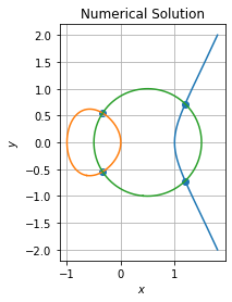
#        [ 1.19616848,  0.71782881]])

That is we have found the four solutions for this problem by intersecting contour curves of zero-level for both implicit equations.

Graphically it renders as follow:

Numerical confirmation

We numerically solve the characteristic polynomial with numpy:

xsol = np.roots([1, 1, -2, -3/4])
# array([-1.85887056,  1.19617217, -0.33730161])

Which are potential solutions for and we assess the coordinate as well:

ysol = np.array([np.sqrt(x ** 3 - x)  for x in xsol])
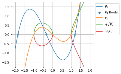
# array([       nan, 0.71787485, 0.54674126])

We can see that only two roots of are real solution for this problem. Hence we have four solutions has we must consider both and .

Graphically it renders as follow:

The precision of those solutions is better but it requires to do algebra by hands where Shapely solved it for use without any knowledge of it.

Alternatively we can also express the system as follow:

def system(x, a, b, x0, y0, r):
    return np.array([
        elliptic(*x, a, b),
        circle(*x, x0, y0, r)
    ])

And solve its roots:

p0 = (-1, 0, 0.5, 0, 1)
sol1 = optimize.fsolve(system, x0=[1,1], args=p0)    # array([1.19617217, 0.71787485])
sol2 = optimize.fsolve(system, x0=[1,-1], args=p0)   # array([ 1.19617217, -0.71787485])
sol3 = optimize.fsolve(system, x0=[-1,1], args=p0)   # array([-0.33730161,  0.54674126])
sol4 = optimize.fsolve(system, x0=[-1,-1], args=p0)  # array([-0.33730161, -0.54674126])

We can plot the distance field:

xlin = np.linspace(-2, 2, 200)
ylin = np.linspace(-2, 2, 200)
X, Y = np.meshgrid(xlin, ylin)
U, V = system([X, Y], *p0)
Z = np.sqrt(U**2 + V**2)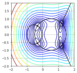

We can confirm than solution of the system are minima of the distance function.