Compute integral using Monte-Carlo

In this post we show how an integral can be computed using Monte-Carlo method and how combination with bootstrapping can increase precision.

Reference

Lets say we wan to integrate the cardinal sinus over the interval . Graphically it is about finding the area under the curve by taking care to respect sign of positive (above x axis) and negative area (below x axis).

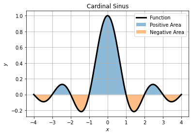
The area of this curve can be numerically computed by trapezoid or quadrature, or analytically.

def model(x):
    return np.sinc(x)

xlin = np.linspace(-4., 4., 20000)
ylin = model(xlin)

Itrap = integrate.trapezoid(ylin, x=xlin)
#  0.9499393464346436

Iquad = integrate.quad(model, xlin.min(), xlin.max())
# (0.9499393397673102, 9.485684460130983e-11)

Both method agrees with the 6 first significant figures and the quadrature value agrees up to its precision to the approximation given by Wolfram Alpha:

   

Method

First we must state the transfer model:

   

Which can be approximated by:

   

The Monte-Carlo method works as follow:

• Uniformly randomly sample points on the domain extent such as ;
• Compute the image of all this points ;
• Estimate the integral using the approximation of the transfer model ;
• Repeat the process time to bootstrap the procedure and let the CLT come into action;

The function below implements such a procedure except bootstrapping:

def monte_carlo(N, a=-1., b=1., model=lambda x: x, seed=12345):
    np.random.seed(seed)
    x = np.random.uniform(a, b, size=N)
    y = model(x)
    return (b - a) / N * np.sum(y)

A single trial gives a poor estimate of the integral, hence the need of bootstrapping:

I = monte_carlo(100000, a=-4., b=4., model=model)
# 0.9491438852706744

Now we will repeat the procedure for different sample size and for each population size we will bootstrap to enhance the estimation:

Nb = 3000
np.random.seed(12345)
estimates = []
for s in np.random.randint(0, 999999999, size=Nb):
    for n in np.logspace(4, 7, 30, base=10).astype(int):
        I = monte_carlo(n, a=-4., b=4., model=model, seed=s)
        estimates.append({"s": s, "n": n, "I": I})
data = pd.DataFrame(estimates)

Once the bootstrap finishes we can aggregate bootstrap samples to see how it helps to converge towards the expected integral value:

agg = data.groupby("n")["I"].agg(["mean", "std"])

Graphically it leads to:

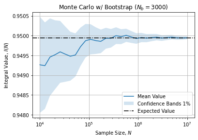
Which shows a convergence towards the expected value when sample increases. Additionally bootstrap samples allows to compute Confidence Bands (here 1%).