Find the closest points to a specific location using KD Tree

In this article we show how KD Tree works and how Voronoi diagram are linked with it by answering a simple question: given a set of reference points (points of interests), find for any point (location) the closet points wrt the reference points set.

import numpy as np
import matplotlib.pyplot as plt
from scipy import spatial

KD Tree

A KD Tree is a binary search tree which split space into sub half-spaces. Using dichotomy search against KD Tree has average search time complexity in which makes KD Tree good option for building spatial search index.

Lets create some random points of interest:

N = 50
pois = np.stack([
    np.random.uniform(0, 1000, size=N),
    np.random.uniform(0, 1000, size=N)
]).T

And create a KDTree with them using scipy.spatial:

kdtree = spatial.KDTree(pois)

Now we create a rectangular grid of location to span the space:

M = 1000
x = np.linspace(0, 1000, M)
y = np.linspace(0, 1000, M)
X, Y = np.meshgrid(x, y)
points = np.stack([X.ravel(), Y.ravel()]).T

We can then query those points against the KD Tree to get a contour map of distances around points of interest:

distances, indices = kdtree.query(points)

Which returns distance and index wrt the closest point of interest for each points of the grid.

D = distances.reshape(X.shape)

fig, axe = plt.subplots(figsize=(7, 7))
contour = axe.contourf(X, Y, D, 50, cmap="viridis")
axe.scatter(*pois.T, marker=".", color="white")
# ...
axe.grid()

Graphically, we can represent the distance wrt to points of interest (seed) as follow:

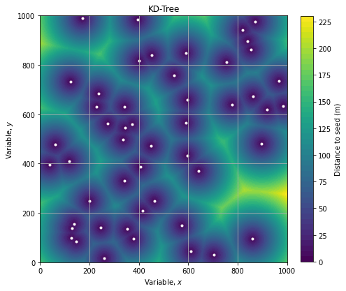
We see a structure like a tiling of the plane which is similar to a Voronoi diagram. It’s a confirmation that our computation are correct.

Voronoi diagram

Voronoi diagram is a partition of a plane into regions around seeds. For each seed (point of interest) there is a corresponding region consisting of all points of the plane closer to that seed than to any other.

We can create such a diagram using scipy.spatial:

voronoi = spatial.Voronoi(pois)

Which renders as follow:

fig, axe = plt.subplots(figsize=(7, 7))
spatial.voronoi_plot_2d(voronoi, ax=axe)
# ...

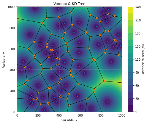
Cell borders are the locus where distance between seeds are equals (tangential circles of same radius).

Querying KD Tree

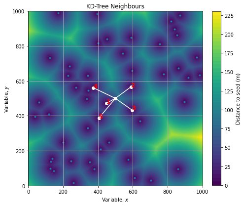
Finding the n-closest neighbours

With KD Tree we can also query the n-closest points wrt a specific location. Lets say we want the 5-closest points wrt the location (500, 500):

location = np.array([500, 500])
dloc, iloc = kdtree.query(location, k=5)
#(array([ 59.31137219, 111.56137442, 115.79092148, 140.73090911, 147.51366679]),
# array([11, 23, 18, 10, 34], dtype=int64))

Where first vector contains distances and second are the indices of point of interest. We can check visually that those 5 points are the closest to the location:

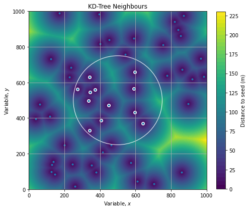
Finding points within a given radius

We can also query the KD Tree to return points within a radius:

iloc2 = kdtree.query_ball_point(location, 250)
# [28, 5, 34, 11, 18, 38, 39, 35, 10, 47, 48, 23]

Which returns the indices of points withing a radius of 250 wrt location: