In this article we show how to symbolically and numerically solve a system of non linear ODE.
Introduction
Given the following system of non linear ODE:
(1) 
With the following parameters:
![]()
Solving the system is about:
- Finding equilibrium states and qualify them;
- Finding time dependent solutions for some given initial values (IVPs);
- Sketch the phase diagram and represent solutions on it.
Analytical solution
First of all we need to find out fixed points of the system. We will use sympy, the python symbolic solver to perform the algebra for us.
If we naively solve the system, we get three fixed points (notice imaginary parts are close to zero):
import sympy as sp
from sympy.abc import N, M, alpha, gamma, epsilon, mu, r, K, rho, theta

parameters = [(alpha, 4 / (K - epsilon) ** 2), (K, 17.3), (epsilon, 4.9), (r, 2.7), (mu, 0.9), (gamma, 3.2)]

h1 = gamma * N / (1 + N) - mu * M
h2 = alpha * r * N ** 2 / (M + N) * (K - N) * (N - epsilon) - mu * N

sp.solve([
    sp.Eq(h1.subs(parameters), 0),
    sp.Eq(h2.subs(parameters), 0),
], [M, N], dict=True)

# [{M: 3.09160042546821, N: 6.66357633525072 + 0.e-22*I},
#  {M: 3.34502350303397 + 6.7762635780344e-21*I, N: 15.8884286880308 - 0.e-20*I},
#  {M: 13.6564215102769 - 1.0842021724855e-19*I, N: -1.35200502328156 - 0.e-22*I}]
Which is a good start (also confirmed by Wolfram Alpha), but misses a potential fixed point at ![]() . Lets investigate a bit more…
. Lets investigate a bit more…
First we isolate ![]() from the second equation:
from the second equation:
![]()
Then we substitute ![]() in first equation, we get:
in first equation, we get:
![]()
For ![]() , the numerator must be null, which gives us a fourth degree polynomial to solve:
, the numerator must be null, which gives us a fourth degree polynomial to solve:
![]()
For the given set of parameters, it leads to:
![]()
Where ![]() is indeed a solution of the polynomial.
is indeed a solution of the polynomial.
Now we need to check the second equation behaves properly at ![]() . We perform the polar transformation and take the limit when radius is going towards zero:
. We perform the polar transformation and take the limit when radius is going towards zero:
![]()
In any direction ![]() .
.
All those computation can be done using sympy:
s = sp.solve(h2, M)
f = sp.simplify(h1.subs(M, s[0]))
n, d = sp.fraction(f)
p = sp.collect(sp.expand(n), N)
p0 = p.subs(parameters)
sol = sp.solve(p0, N)

# [0.0,
#  -1.35200502328156 + 0.e-22*I,
#  6.66357633525071 - 0.e-22*I,
#  15.8884286880309 + 0.e-22*I]

h2p = h2.subs({M: rho * sp.sin(theta), N: rho * sp.cos(theta)})
h2p.limit(rho, 0)  # 0
Defining the model
Lets import the required libraries. Then we define a set of parameters for a given dynamic and define the model as a system of equations:
import numpy as np
import numdifftools as nd
from scipy import integrate, optimize, linalg
import matplotlib.pyplot as plt

prop_cycle = plt.rcParams['axes.prop_cycle']
colors = prop_cycle.by_key()['color']

K = 17.3
epsilon = 4.9
r = 2.7
mu = 0.9
gamma = 3.2
alpha = 4 / (K - epsilon) ** 2

p0 = (alpha, r, K, epsilon, mu, gamma)

def model(t, y, alpha, r, K, epsilon, mu, gamma):
    return np.array([
        gamma * y[1] / (1 + y[1]) - mu * y[0],
        alpha * r * (y[1] ** 2 / (y[1] + y[0])) * (K - y[1]) * (y[1] - epsilon) - mu * y[1]
    ])
Finding fixed points
First we create grids for our variables and compute the vector fields associated to the ODE system. We also create a proxy method that match the optimize.root signature to finds roots of the field. Finally we solve the system of equations for initial educated guess:
Mlin = np.linspace(-10, 15, 1000)
Nlin = np.linspace(-5, 20, 1000)
M, N = np.meshgrid(Mlin, Nlin)

t = np.linspace(2, 10, 200)

U, V = model(t, [M, N], *p0)
C = np.sqrt(U ** 2 + V ** 2)

def proxy(x):
    return model(None, x, *p0)

sol0 = optimize.root(proxy, x0=[1, 1])       # [ 1.976e-323  4.941e-324]
sol1 = optimize.root(proxy, x0=[5, 7.5])     # [ 3.092e+00  6.664e+00]
sol2 = optimize.root(proxy, x0=[2.5, 17.5])  # [ 3.345e+00  1.589e+01]
sol3 = optimize.root(proxy, x0=[13, -1.5])   # [ 1.366e+01 -1.352e+00]

fig, axe = plt.subplots()
axe.contour(M, N, np.log10(C), 20, cmap="viridis")
for sol in [sol0, sol1, sol2]:
    axe.scatter(*sol.x, color="blue")
axe.grid()

fig, axe = plt.subplots()
axe.contour(M, N, U, [0], colors=colors[0])
axe.contour(M, N, V, [0], colors=colors[1])
for sol in [sol0, sol1, sol2, sol3]:
    axe.scatter(*sol.x, color="blue")
axe.grid()
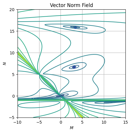
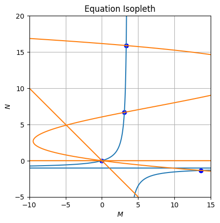
Looking at the vector norm field or the equation isopleths, we can identify four fixed points as we found when solving analytically the problem:


Nature of fixed points
In order to get the nature of the fixed points we need to assess the eigenvalues of the Jacobian of the system at each fixed point. This can be done using numdifftools and scipy:
eigenvalues = []
for sol in [sol0, sol1, sol2, sol3]:
    J = nd.Jacobian(proxy)(sol.x)
    e, v = linalg.eigh(J)
    eigenvalues.append(e)

# [array([-6.85418835, -0.9       ]),  # Attractor
#  array([-0.9918713 ,  3.21386104]),  # Repellor
#  array([-8.74288298, -0.82952149]),  # Attratcor
#  array([-0.90452072,  1.26327589])]  # Repellor
We find that two fixed points are attractors and the two other are repellors.
Solving the dynamic
Now we solve some IVPs to see how they get attracted or repulsed by the fixed points.
M0 = 5.6667
N0 = K / 1.5

y0 = (M0, N0)
y1 = (4, 6)
y2 = (10, 2.5)

ivp0 = integrate.solve_ivp(model, [t.min(), t.max()], args=p0, y0=y0, t_eval=t, atol=1e-8, rtol=1e-8)
ivp1 = integrate.solve_ivp(model, [t.min(), t.max()], args=p0, y0=y1, t_eval=t, atol=1e-8, rtol=1e-8)
ivp2 = integrate.solve_ivp(model, [t.min(), t.max()], args=p0, y0=y2, t_eval=t, atol=1e-8, rtol=1e-8)

fig, axe = plt.subplots()
for ivp, color in zip([ivp0, ivp1, ivp2], colors[:3]):
    axe.plot(t, ivp.y[0], "-", color=color)
    axe.plot(t, ivp.y[1], "--", color=color)
axe.grid()
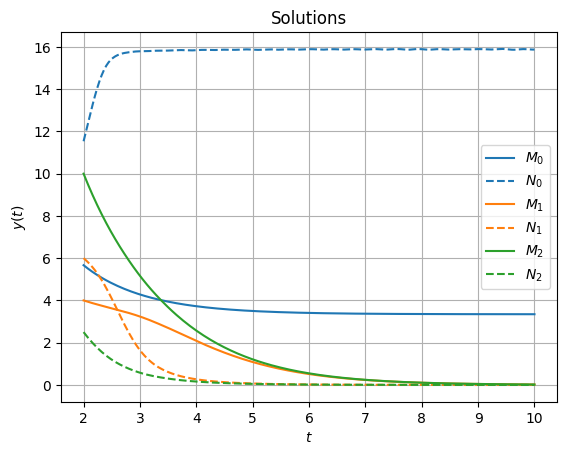
Those time dependents solutions looks like:

Now we can plot those solutions over a stream plot:
fig, axe = plt.subplots()
axe.streamplot(M, N, U, V, color="grey")
for sol in [sol0, sol1, sol2, sol3]:
    axe.scatter(*sol.x, marker="o", color="blue")
axe.plot([-10, 5], [10, -5], "--", color="black")
axe.plot([-10, 15], [-1, -1], "--", color="black")
for y, ivp, color in zip([y0, y1, y2], [ivp0, ivp1, ivp2], colors[:3]):
    axe.scatter(*y, color=color)
    axe.plot(*ivp.y, color=color)
axe.grid()
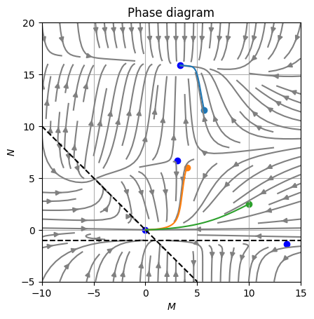
Which renders as follow:

As we can see the numerical approach is compliant with the analytical solution and provides more insight of the dynamic behavior of the solution.
