Revisiting the Michaelis-Menten model

This post revisits the Michaelis-Menten model.

Model

The Michaelis-Menten model assumes the following reactions:

$E + S \underset{k_{-1}}{\overset{k_1}{\rightleftharpoons}} ES \overset{k_{cat}}{\rightarrow} E + P$

Where:

$E$ is the Enzyme that catalyses the overall reaction;
$S$ is the Substrate consumed by the overall reaction;
$ES$ is the complex Enzyme-Substrate (intermediate state);
$P$ is the Product of the overall reaction.

If we assume the law of mass action for those two elementary reactions, we get the following kinetic laws:

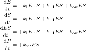
(1) $\begin{align*}\frac{\mathrm{d}E}{\mathrm{d}t} &= - k_1 E \cdot S + k_{-1} ES + k_{cat} ES \\\frac{\mathrm{d}S}{\mathrm{d}t} &= - k_1 E\cdot S + k_{-1} ES \\\frac{\mathrm{d}ES}{\mathrm{d}t} &= + k_1 E\cdot S - k_{-1} ES - k_{cat} ES \\\frac{\mathrm{d}P}{\mathrm{d}t} &= + k_{cat} ES\end{align*}$

Which describes the dynamic of the reactions.

Simplifications

For specific experimental setup, it is possible to apply some simplifications.

Enzyme is a catalyst

First of all, $E$ is a catalyst, therefore it is not consumed by the overall reaction and can be added in small proportion wrt the substrate. Assuming the Substrate concentration $S$ is several order of magnitude higher than the Enzyme concentration $E$ such as $E \ll S$ allows us to deduce that $ES \ll S$ and therefore $S$ is almost constant during a small time span.

Steady state approximation

When the equilibrium is reached (assumed to be quick), because the concentration of substrate $S$ is almost constant and the Enzyme is not consumed, we may assume that the Enzyme-Substrate concentration $ES$ is constant over time. That is:

$\frac{\mathrm{d}ES}{\mathrm{d}t} = 0$

Enzyme is stable and specific

The Enzyme is stable (it is not destructed over time) and specific (it only binds with the Substrate not the Product). Therefore the following mass balance can be derived:

$E_{tot} = E + ES$

Definitions

For convenience we also define two quantities, such as:

(2) $\begin{align*}k_M &= \frac{k_{-1} + k_{cat}}{k_1} \\v_\max &= k_2 E_{tot}\end{align*}$

Where $k_M$ is the Michaelis-Menten constant and $v_\max$ is the maximal theoretical Product rate when all Enzyme is in the form of the Enzyme-Substrate complex.

Michaelis-Menten law

If we apply the simplifications to the model, we can draw the following relation:

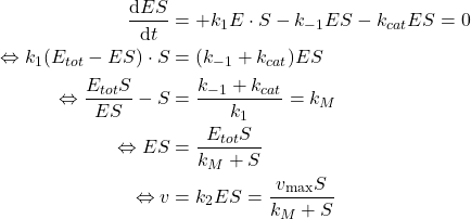
(3) $\begin{align*}\frac{\mathrm{d}ES}{\mathrm{d}t} &= + k_1 E\cdot S - k_{-1} ES - k_{cat} ES = 0 \\\Leftrightarrow k_1 (E_{tot} - ES)\cdot S &= (k_{-1} + k_{cat}) ES \\\Leftrightarrow \frac{E_{tot}S}{ES} - S &= \frac{k_{-1} + k_{cat}}{k_1} = k_M \\\Leftrightarrow {ES} &= \frac{E_{tot}S}{k_M + S} \\\Leftrightarrow v &= k_2 ES = \frac{v_{\max} S}{k_M + S}\end{align*}$

The drawn relation implies is only dependent of the experimental setup $v_\max$ (hence $E_{tot}$ ) and related kinetic constants $k_1$ , $k_{-1}$ and $k_{cat}$ and the Substrate concentration $S$ .

Lineweaver-Bürk Linearization

Finally, notice than the Michaelis-Menten law can be linearized by taking the inverse of the equation:

(4) $\begin{align*}v &= \frac{v_{\max} S}{k_M + S} \\\Leftrightarrow \frac{1}{v} &= \frac{k_M}{v_\max}\frac{1}{S} + \frac{1}{v_\max}\end{align*}$

Which allows us to perform linear regression on $\left(\frac{1}{v}, \frac{1}{S}\right)$ .

Solving the dynamic

Lets solve the dynamic for a typical setup where the simplifications apply.

import numpy as np
import matplotlib.pyplot as plt
from scipy import optimize, integrate, special

def model(t, x, k1, k1inv, kcat):
    return np.array([
        - k1 * x[0] * x[1] + k1inv * x[2] + kcat * x[2],
        - k1 * x[0] * x[1] + k1inv * x[2],
        + k1 * x[0] * x[1] - k1inv * x[2] - kcat * x[2],
        + kcat * x[2]
    ])

t = np.linspace(0, 1000, 200)
x0 = np.array([1e-6, 1e-1, 0.0, 0.0])
ks = np.array([1e-1, 1e-2, 1e-3])

solution = integrate.solve_ivp(model, [t.min(), t.max()], y0=x0, args=ks, t_eval=t, atol=1e-16, rtol=1e-12)

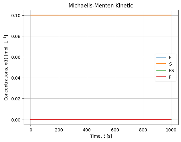
The overall solutions looks like:

If we zoom on the smaller concentrations, it looks like:

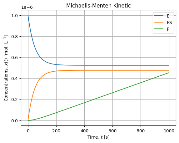
We confirm our simplification hypothesis:

Substrate concentration is several decade higher than other concentration, it is almost constant over the experiment;
When equilibrium is established, the production rate is constant (linear kinetic).

Checking the Michaelis-Menten law

At this point, we can check the agreement of the drawn Michaelis-Menten law with our numerical experiment. What we need to do is: find terminal rates of reaction of several Substrate concentration to see if they follow the model we have derived.

Ss = np.linspace(0, 1, 25)

vs = []
sols = []
for S in Ss:
    x0 = np.array([1e-6, S, 0.0, 0.0])
    solution = integrate.solve_ivp(system, [t.min(), t.max()], y0=x0, args=ks, t_eval=t, atol=1e-16, rtol=1e-12)
    sols.append(solution)
    v = system(t, solution.y, *ks)
    vs.append(v[3,-1])
vs = np.array(vs)

def model(x, vmax, kM):
    return vmax * x / (x + kM)

popt, pcov = optimize.curve_fit(model, Ss, vs)
# [1.00000112e-09, 1.10001135e-01]

vhat = model(Ss, *popt)

We first check that for all Substrate concentration the equilibrium is reached:

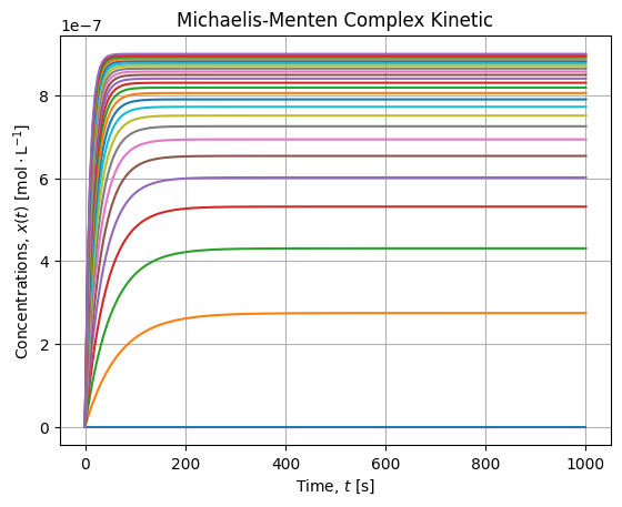
It is the case, 1000 [s] seems to be sufficient to settle the equilibrium. Then we can plot final rates wrt Substrate concentrations and check the fit agreement with the Michaelis-Menten model:

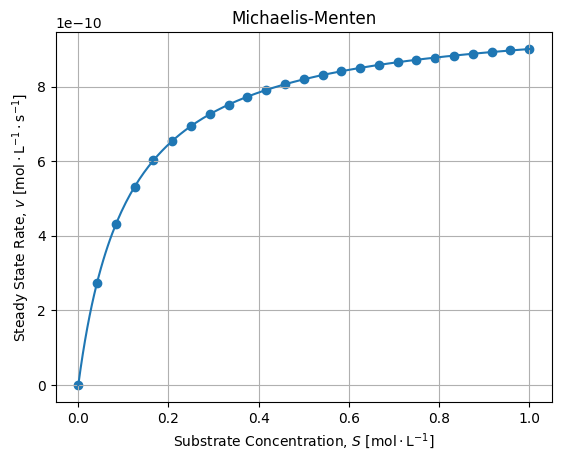
The adjustment is fair. If we compute relative error between numerical solutions of the dynamic and Michaelis-Menten adjustment we get the following error:

$e_r(v) = \frac{\hat{v} - v}{v}$

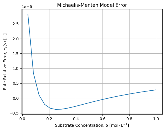
We see the error is structured but acceptable. We confirm that the model diverges when the Substrate concentrations are low, say cannot be considered largely superior wrt the Enzyme concentration. The sign of the error also provides an interesting information: when Substrate concentration is low, the Michaelis-Menten over estimate $\hat{v}$ before the exact solution $v$ .

If we compare regressed values with expected values we get:

vmax = ks[2] * x0[0]          # 1e-9
kM = (ks[1] + ks[2]) / ks[0]  # 0.10999999999999999

Seems acceptable for this application, anyway we may quote George Box:

All models are wrong, some are useful.

Which is the case for the Michaelis-Menten law provided we stick to its hypothesis.

Linearization

We can perform the Lineweaver-Burk linearization of our exact solutions and check it fits a regular straight line:

poptL, pcovL = optimize.curve_fit(linear, 1 / Ss[1:], 1 / vs[1:])
vmaxL =  1./ poptL[1]   # 1.0000021367938439e-09
kML = poptL[0] * vmaxL  # 0.11000162856713572

If we draw linearization of numerical solutions, we get:

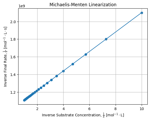
It confirms Lineweaver-Burk linearization is effective for linearizing Michaelis-Menten law.

Analytical solution

If the assumption than the equilibrium is almost instantaneous, there is an analytical solution for the Michaelis-Menten equation allowing to draw an explicit expression for $S(t)$ :

(5) $\begin{align*}v = \frac{\mathrm{d}P}{\mathrm{d}t} = \frac{v_{\max} S}{k_M + S} &\simeq -\frac{\mathrm{d}S}{\mathrm{d}t} \\\Leftrightarrow\int\limits_{S_0}^S \frac{k_M + S}{S} \mathrm{d}S &= -\int\limits_0^t v_{\max} \mathrm{d}t \\\Leftrightarrow\left[k_M\ln(S) + S\right]_{S_0}^S &= \left[- v_{\max} t\right]_0^t \\\Leftrightarrow\ln\left(\frac{S}{S_0}\right) + \frac{S - S_0}{k_M} &= -\frac{v_{\max} t}{k_M} \\\Leftrightarrow\frac{S}{k_M} \exp\left(\frac{S}{k_M}\right) &= \frac{S_0}{k_M}\exp\left(\frac{S_0 - v_{\max} t}{k_M}\right) \\\Leftrightarrow S &= k_M W_0 \left[\frac{S_0}{k_M}\exp\left(\frac{S_0 - v_{\max} t}{k_M}\right)\right]\end{align*}$

Where $W_0$ is the first branch of the Lambert function. We can confirm the math with sympy or Wolfram:

import sympy as sp
from sympy.abc import k, t, s, v 

s0 = sp.Symbol("s0")
h1 = sp.integrate((k + s) / s, (s, s0, s))
h2 = sp.integrate(-v, (t, 0, t))
sol = sp.solve(sp.Eq(h1, h2), s)
# [k*LambertW(s0*exp((s0 - t*v)/k)/k)]

If we draw this solution compared to our dynamic model we get the following curves:

def S(t, S0, vmax, kM):
    return np.real(kM * special.lambertw(S0 / kM * np.exp((S0 - vmax * t) / kM)))

s = S(t, 1, vmax, kM)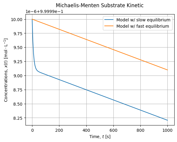

We see there is a small bias between the ODE Solution with a slow equilibrium and the analytical solution we have drawn that assumes the equilibrium is instantaneous. Anyway the slope of the kinetic are alike when the equilibrium is reached. Meaning the curves will converges for fast equilibrium. Also notice the small scale of this evolution which is about $10^{-6}$ .