Fit implicit function

This post reviews how to fit an implicit function using the scipy package.

import numpy as np
import matplotlib.pyplot as plt
from scipy import optimize

Sketching the function

First, lets sketch the function. Assume we have the following implicit function (here an elliptic curve):

def model(x, y, a=-2., b=+0.5):
    return x ** 3 + a * x + b - y ** 2

We can draw the function using contour with a level of zero:

xlin = np.linspace(-5, 5, 200)
ylin = np.linspace(-5, 5, 200)
X, Y = np.meshgrid(xlin, ylin)
Z = model(X, Y)

fig, axe = plt.subplots()
c = axe.contour(X, Y, Z, [0])  # Zero isopleth is indeed the solution of the equation

Which renders as follow:

Generating dataset

We can use the contour drawn in previous step to extract a dataset of such an implicit function:

data = c.get_paths()[0].vertices
data += 0.1 * np.random.normal(size=data.shape)

We also add a bit of noise on it, to make things crispier.

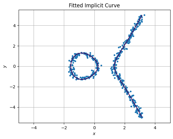
Fitting the curve

Now we have the model and the dataset, we can fit the model to the dataset by writing an appropriate loss function to minimize. We write the following factory and loss function:

def loss_factory(x, y):
    def wrapped(parameters):
        return 0.5 * np.sum(model(x, y, *parameters) ** 2)
    return wrapped

loss = loss_factory(*data.T)

Now everything is setup to minimize the loss function and regress the implicit curve parameters:

sol = optimize.minimize(loss, x0=[1, 1])

#  message: Optimization terminated successfully.
#  success: True
#   status: 0
#      fun: 373.14780914303003
#        x: [-2.099e+00  4.963e-01]
#      nit: 5
#      jac: [ 0.000e+00  0.000e+00]
# hess_inv: [[ 9.784e-04 -1.055e-03]
#            [-1.055e-03  3.385e-03]]
#     nfev: 27
#     njev: 9

The results of the adjustments looks like: