Understanding PCA and implementing it step by step using python

This post details how principal component analysis (PCA) works and how to perform it step by step using Python.

Mathematics behind PCA

First we state the mathematical basis of PCA in order to get the full picture before applying it to real data.

Data decomposition

Consider the real matrix of observations of dimension, it’s always possible to decompose it into it’s Singular Value Decomposition ‐ which is a generalization of eigendecomposition ‐ as follow:

   

Or in its reduced form:

   

Where:

• are principal components normalized to unit norm ( is a unitary matrix);
• are singular values ( is a diagonal matrix);
• are singular vectors ( is an orthogonal matrix, and is an orthonormal basis of principal components space).

Covariance decomposition

Consider the covariance matrix defined as follow:

   

Where is necessarily centered to origin (mean of each column is zero).

Using the SVD decomposition defined above, the covariance matrix can be expressed as:

   

Which proves the covariance matrix is eigen-decomposable and has the same orthonormal basis than the SVD of the data matrix . The relation between singular values and the eigen values is then defined as .

Also, notice:

• by transposition;
• because is diagonal;
• because is unitary;
• because is orthogonal.

Variance conservation

A nice property of PCA is it conserves the total variance of the dataset. Covariance matrix is real symmetric and therefore by the spectral theorem it is diagonalizable.

   

Notice than trace for matrix commutation are equals .

Which proves that the total variance of the dataset is conserved and is equal to the sum of eigenvalues.

Principal components

Principal components are the projection of observations in into the principal components space defined by the columns of . Performing the change of basis leads to:

   

Principal components are the unitary principal components scaled by singular values by decreasing order of magnitude.

This is where PCA becomes useful. Because it allows to capture a maximum of variance in the very first dimensions of its principal components. Therefore dimensionality of dataset can be reduced while keeping a maximum of information. This can be assimilated to a compression.

PCA Loadings

Lets define standardized principal components as follow:

   

Loadings can be defined as the covariance between data matrix and standardized principal components :

   

Warning: definition of loadings are not universal and generally depends on software implementation. For instance, the definition above has been chosen for its clean mathematical point of view. Although it is a common definition, there are software (such as R) which compute loadings in a different way.

PCA, step by step

First, lets import some modules and a dataset to shoulder our computations:

import numpy as np
import pandas as pd
import matplotlib.pyplot as plt
import seaborn as sns
from scipy import linalg

data = sns.load_dataset("iris")
target = data.pop("species")
X = data.values

Detailed computations and sanity checks

We center the dataset (required):

n, k = X.shape        # (150, 4)
Xm = X.mean(axis=0)   # [5.84333333, 3.05733333, 3.758     , 1.19933333]
X -= Xm

We also compute the standard deviation and the total variance:

Xs = X.std(axis=0, ddof=1)  # [0.82806613, 0.43586628, 1.76529823, 0.76223767]
Vx = np.sum(Xs ** 2)        # 4.572957046979866

From X we can compute the Covariance matrix and check it is symmetric and positive definite:

C = X.T @ X / (n - 1)

np.allclose(C, C.T)            # True
np.all(linalg.eigvals(C) > 0)  # True
linalg.cholesky(C)             # Exists

Now we can perform the SVD and confirm the decomposition is correct:

U, s, Vt = linalg.svd(X, full_matrices=False)
S = np.diag(s)
V = Vt.T

np.allclose(X, U @ S @ Vt)  # True

We can also confirm matrices are unitary/orthogonal:

np.allclose(np.eye(k), U.T @ U)  # True
np.allclose(np.eye(k), V.T @ V)  # True
np.allclose(V.T, linalg.inv(V))  # True

Also notice than matrix U is centered to origin and normalized by columns:

np.mean(U, axis=0)      # [0., 0., 0., 0.]
linalg.norm(U, axis=0)  # [1., 1., 1., 1.]

We confirm variance is conserved (redistributed among eigenvalues):

E = S ** 2 / (n - 1)
np.allclose(Vx, np.sum(E))  # True

Now we can perform the projection into the principal components space:

Z = X @ V

np.allclose(Z, U @ S)  # True

And finally we can compute loadings:

Y = np.sqrt(n - 1) * U
L = V @ S / np.sqrt(n - 1)

np.allclose(L, X.T @ Y / (n - 1))  # True

Summary

Now we can summarize the whole operation into these few lines:

U, s, Vt = linalg.svd(X, full_matrices=False)
S = np.diag(s)
V = Vt.T
E = S ** 2 / (n - 1)
Z = U @ S
L = V @ S / np.sqrt(n - 1)

The same goal can be achieved with sklearn:

from sklearn.decomposition import PCA

pca = PCA()
pca.fit(X)

V = pca.components_.T
E = np.diag(pca.explained_variance_)
L = V @ np.sqrt(E)

Visualizations

Two figures are generally associated with PCA: Variance Plot and Bi Plot.

The first figure shows how the variance is distributed among the principal components and is used to help to find the right amount of dimension to keep.

c = np.arange(k)
rVx = np.diag(E) / Vx
SrVx = np.cumsum(rVx)

from matplotlib.ticker import MaxNLocator

fig, axe = plt.subplots()
axe.bar(c, rVx, alpha=0.7)
axe.plot(c, SrVx, "-o")
for i in c:
    axe.text(c[i], SrVx[i], "%.3f" % SrVx[i])
axe.set_title("PCA: Variance Explained")
axe.set_xlabel("Principal Components Index")
axe.set_ylabel("Variance explained")
axe.xaxis.set_major_locator(MaxNLocator(integer=True))
axe.grid()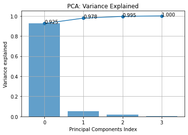

In this example, we see that if we keep the two first component we capture at least 97.8% of the variance, which is totally acceptable.

The second figure shows the data projected into the reduced principal components space and how each variable contributes to each component (loadings):

fig, axe = plt.subplots()
for key in target.unique():
    q = target == key
    axe.scatter(*Z[q, :2].T, label=key)
for i in range(k):
    axe.arrow(0, 0, *L[i, :2])
    axe.text(*L[i, :2], str(i))
axe.set_title("PCA: Bi Plot")
axe.set_xlabel("")
axe.set_ylabel("")
axe.legend()
axe.grid()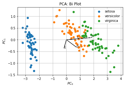

In this example, we see the two first components and loadings according to our definition. This figure allows us to see clusters in the dataset by taking the best snapshot of it (projection with more explained variance).

Loadings inform us than the first variable contributes to both components, while second variable contributes more to the second component, finally third and fourth variables mainly contribute to the first principal component.