This post reviews a classical catalytic reaction kinetic and multiple ways to adjust it to experimental dataset. We will see that modern computer can solve the kinetic symbolically and numerically while old fashion methods also provides good results.
Model
We want to model an heterogeneous reaction between Isopropanol and Raney’s Nickel which is a catalytic deshydrogenation. Reaction produces Isopropanone (acetone) and dihydrogen:
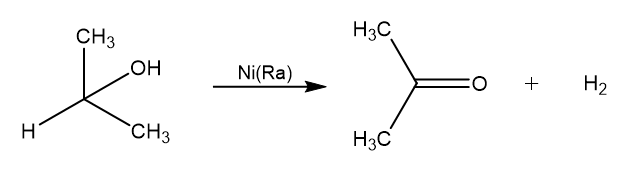
For sake of simplicity we label the reaction as follow:
![\[\mathrm{A \underset{Ni}{\overset{k_1}{\longrightarrow}} B + C}\]](https://landercy.be/wp-content/ql-cache/quicklatex.com-d6295475542ef868b21f68d5f0152e3e_l3.png "Rendered by QuickLaTeX.com")
Where  is the kinetic constant of the reaction which is governed by chimisorption of reactant and products on the catalyst surface. Using the Langmuir isothermal model for monosorption the kinetic can be modelled follow:
![\[r = k_1 \theta_A = k_1\frac{aA}{1 + aA + bB + cC}\]](https://landercy.be/wp-content/ql-cache/quicklatex.com-3a022f71f16a41b7c65b7b9a62e9c3f3_l3.png "Rendered by QuickLaTeX.com")
By taking an ad hoc experimental setup (solution bulk is pure Isopropanone, hydrogen is continuously withdrawn from the system) we can simplify this model to:
![\[r = \frac{1}{V}\frac{\mathrm{d}\xi}{\mathrm{d}t} \simeq k_1\frac{aA}{aA + bB} = k_1\frac{a(n_0 - \xi)}{a(n_0 - \xi) + b\xi}\]](https://landercy.be/wp-content/ql-cache/quicklatex.com-5d9e1c84597e7cc8f3df7f0419a76b24_l3.png "Rendered by QuickLaTeX.com")
Where  is the reaction coordinate and
  are reactant and product respective affinities for the catalyst surface. This ODE is separable:
![\[\int\limits_0^\xi\left(1 + \frac{b\xi}{a(n_0-\xi)}\right)\mathrm{d}\xi = \int\limits_0^t k_1 V\mathrm{d}t\]](https://landercy.be/wp-content/ql-cache/quicklatex.com-be1c4e1e66583e1babb41ed0958f57c4_l3.png "Rendered by QuickLaTeX.com")
We define  as the ratio of product/reactant affinity constants. Integration leads to an explicit function for time w.r.t reaction coordinate:
![\[\left(1 - k_2\right)\xi - k_2 n_0 \ln\left(\frac{n_0 - \xi}{n_0}\right) = k_1 V t\]](https://landercy.be/wp-content/ql-cache/quicklatex.com-87aa14c3fe819d325c425a058f53fde6_l3.png "Rendered by QuickLaTeX.com")
We can make this relation explicit for reaction coordinate using the Lambert function. Inversion leads to:
![\[\xi &= n_0 \left( 1 - \frac{k_2}{1 - k_2}W_0\left[\frac{1 - k_2}{k_2}\exp\left(- \frac{k_1 V t}{n_0 k_2} + \frac{1 - k_2}{k_2} \right) \right] \right)\]](https://landercy.be/wp-content/ql-cache/quicklatex.com-807ef4f34cd671f23da29d558598c9d9_l3.png "Rendered by QuickLaTeX.com")
Which may be undefined when  . Solving the limits using L’Hopsital rule gives:
![\[\lim\limits_{k_2 \rightarrow 1} \xi = n_0 \left(1 - \exp\left(-\frac{k_1 V t}{n_0}\right)\right)\]](https://landercy.be/wp-content/ql-cache/quicklatex.com-8568e767ba50a0e19fb509f1daf4e7be_l3.png "Rendered by QuickLaTeX.com")
Based on this model we can assess the two chemical constants and  by monitoring the reaction kinetic simply by logging produced hydrogen volume as a function of time.
For a typical setup and a unitary constant, figure below shows how profile varies with :
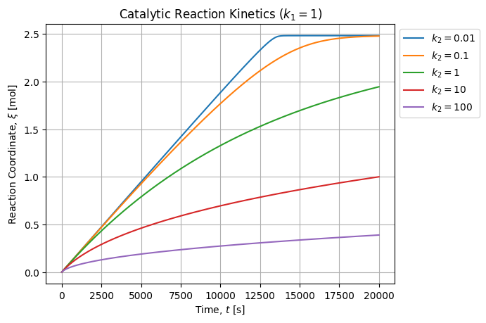
As expected when  the kinetic is slowed down because the product poisons the catalyst by removing reactive site fraction available for reaction. When
  , the kinetic is almost linear until all the reactant is consumed because the active surface remains almost constant. When we are in the case where the analytical model reduces to a classical exponential profile.
Symbolic checks
We can confirm our manual computations using the sympy library:
import sympy as sp

t, xi, k1, k2, n, V = sp.symbols("t xi k1 k2 n V")

g1 = 1 + k2 * xi / (n - xi)
g2 = k1 * V

h1 = sp.integrate(g1, (xi, 0, xi))
h2 = sp.integrate(g2, (t, 0, t))

sol = sp.solve(sp.Eq(h1, h2), xi)
# [n*(k2*LambertW((1 - k2)*exp((-V*k1*t - k2*n + n)/(k2*n))/k2) + k2 - 1)/(k2 - 1)]

sp.expand(sp.limit(sol[0], k2, 1))
# n - n*exp(-V*k1*t/n)
Using Wolfram Alpha, we can also confirm the inversion and the limit case. We are confident our model is correct provided our hypothesis.
Alternative methods
The explicit solution  requires to have access to the Lambert W function in the software you are using to perform calculation. This is not the case of Excel for instance and it also provided another cost before computer even existed. Therefore alternative methods exist to solve this kinetic, we show two of them in this section.
Ordinary Least Squares
The explicit function  is linear in term of parameters and therefore can be solved by Ordinary Least Squares method:
![\[t(\xi) = \frac{1}{k_1}(1-k_2) \frac{\xi}{V} + \frac{k_2}{k_1}\left(-\frac{n_0}{V}\right)\ln\left(\frac{n_0 - \xi}{n_0}\right) = c_1 x_1(\xi) + c_2 x_2(\xi)\]](https://landercy.be/wp-content/ql-cache/quicklatex.com-b3774be43a38603271e6f3a8d7d5db67_l3.png "Rendered by QuickLaTeX.com")
Where:
![\[x_1(\xi) = \frac{\xi}{V}, \quad x_2(\xi) = -\frac{n_0}{V}\ln\left(\frac{n_0 - \xi}{n_0}\right)\]](https://landercy.be/wp-content/ql-cache/quicklatex.com-f1a9d1cfe89a09790f6622092cddbd47_l3.png "Rendered by QuickLaTeX.com")
Then kinetic constants can be deduced using:
![\[k_1 = \frac{1}{c_1 + c_2} \,,\quad k_2 = \frac{c_2}{c_1 + c_2}\]](https://landercy.be/wp-content/ql-cache/quicklatex.com-55f5c1537fe4add48a32c96689eb8276_l3.png "Rendered by QuickLaTeX.com")
Lineweaver-Bürk Linearization
This is the old-fashion effective solution. We may consider the fact that the inverse of the reaction rate is a straight line wrt to Product/Reactant ratio:
![\[r = k_1\frac{aA}{aA + bB} \rightarrow \frac{1}{r} = \frac{1}{k_1}\left(1 + k_2 \frac{\xi}{n_0 - \xi}\right) = c_3 x_3(\xi) + c_4\]](https://landercy.be/wp-content/ql-cache/quicklatex.com-be883c673e692ce0a10601024ed5b925_l3.png "Rendered by QuickLaTeX.com")
Therefore if we can assess the reaction rate and inverse it, we can perform usual Linear Regression using OLS and regress the kinetic constants:
![\[k_1 = \frac{1}{c_4}, \quad k_2 = \frac{c_3}{c_4}\]](https://landercy.be/wp-content/ql-cache/quicklatex.com-88bbd7a68046d44eaa7178f04fd930d4_l3.png "Rendered by QuickLaTeX.com")
Libraries
Libraries used in this article are:
import numpy as np
import pandas as pd
import matplotlib.pyplot as plt

from scipy import optimize, special
from sklearn import metrics
from sklearn.linear_model import LinearRegression
from sklearn.preprocessing import PolynomialFeatures
Experimental setup
For the given experimental setup:
R = 8.31446261815324           # J/mol.K
T0 = 292.05                    # K
p0 = 101600                    # Pa
V = 190e-6                     # m3 of isopropanol
m = 2.7677                     # g of Raney Nickel
rho = 785                      # kg/m³
M = 60.1                       # g/mol
n0 = 1000 * rho * V / M        # mol
We have collected the following dataset. We compute the reaction coordinate :
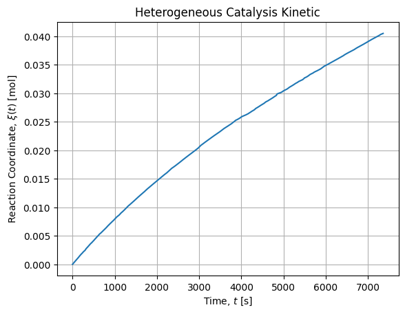
df = pd.read_csv("cathet.csv")
df["xi"] = p0 * df["V"] / (R * T0)
It renders as follow:
Non linear adjustment of direct model
We first solve the direct case and we will use it as a reference to compare other methods.
def model1(t, k1, k2):
    if k2 != 1.:
        return np.real(n0 * (1 - k2 / (1 - k2) * special.lambertw((1 - k2) / k2 * np.exp(- k1 * V * t / (n0 * k2) + (1 - k2) / k2))))
    else:
        return n0 * (1. - np.exp(- (k1 * t * V) / n0))

popt1, pcov1 = optimize.curve_fit(model1, df["t"], df["xi"])
# (array([4.74055853e-02, 7.73469604e+01]),
#  array([[1.03016125e-08, 5.13022024e-05],
#         [5.13022024e-05, 2.64738605e-01]]))

sp1 = np.sqrt(np.diag(pcov1))
# array([1.01496860e-04, 5.14527555e-01])

df["xi1"] = model1(df["t"], *popt1)
score1 = metrics.r2_score(df["xi"], df["xi1"])
# 0.9999564205718714
The adjustment seems fair and renders as follow:
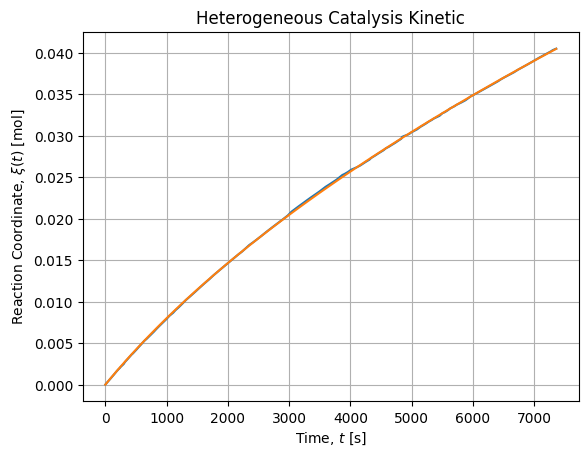
Our reference parameters drawn from this reference are ![k_1 = (4.74 \pm 0.01) \times 10^{-2} [\mathrm{mol \cdot m^{-3} \cdot s^{-1}}]](https://landercy.be/wp-content/ql-cache/quicklatex.com-09411af69b2e062e30b6dbbecb3c4eb9_l3.png "Rendered by QuickLaTeX.com") and
and ![k_2 = (7.73 \pm 0.05) \times 10^{1} [-]](https://landercy.be/wp-content/ql-cache/quicklatex.com-f19c241b72ccd45dbe5ff0b04306f756_l3.png "Rendered by QuickLaTeX.com") . We are in the case where the product has more affinity for the surface than the reactant leading to a poisoning.
. We are in the case where the product has more affinity for the surface than the reactant leading to a poisoning.
Linear adjustment of reverse model
If we don’t have access to the Lambert W function but we have access to a multi-dimensional Ordinary Least Squares solver, then we can perform the following regression:
df["x1"] = df["xi"] / V
df["x2"] = - (n0 / V) * np.log((n0 - df["xi"]) / n0)

X3 = df[["x1", "x2"]].values
y3 = df["t"].values

OLS3 = LinearRegression(fit_intercept=False).fit(X3, y3)

def solveOLS3(c1, c2):
    k1 = 1. / (c1 + c2)
    k2 = c2 * k1
    return np.array([k1, k2])

popt3 = solveOLS3(*OLS3.coef_)
# array([4.75360719e-02, 7.80055911e+01])

df["xi3"] = model1(df["t"], *popt3)
score3 = metrics.r2_score(df["xi"], df["xi3"])
# 0.9999557843907094
Regressed parameters are similar to the reference and the score is almost as good as the reference.
Lineweaver-Bürk Linearization
If we only have simple linear regression as an option, then we may resort to Lineweaver-Bürk Linearization. The only constraint is to be able to assess the rate of reaction in order to get its inverse.
Crude first difference
A naive and noisy way to estimate reaction rate is to assess the first differences ratio:
df["B/A"] = df["xi"] / (n0 - df["xi"])
df["dxidt1"] = df["xi"].diff() / df["t"].diff()
df["1/r1"] = V / df["dxidt1"]

X4 = df[["B/A"]].values[1:]
y4 = df["1/r1"].values[1:]

OLS4 = LinearRegression(fit_intercept=True).fit(X4, y4)

def solveOLS4(ols):
    k1 = 1 / ols.intercept_
    k2 = ols.coef_[0] * k1
    return np.array([k1, k2])

popt4 = solveOLS4(OLS4)
# array([4.70185573e-02, 7.82451296e+01])

df["xi4"] = model1(df["t"], *popt4)
score4 = metrics.r2_score(df["xi"], df["xi4"])
# 0.999623288775574
Polynomial smooth first difference
Because derivation and first difference are very sensitive to noise, we may want to smooth out our kinetic profile before applying first difference method. We pick a cubic interpolation method as it is available in Excel default fitting toolbox.
X5P = df[["t"]].values
y5P = df["xi"].values

XP5 = PolynomialFeatures(degree=3).fit_transform(X5P)
OLS5P = LinearRegression(fit_intercept=False).fit(XP5, y5P)
y5Phat = OLS5P.predict(XP5)

dCdt5 = np.diff(y5Phat) / df["t"].diff().values[1:] / V
X5 = df[["B/A"]].values[1:,:]
y5 = 1. / dCdt5

OLS5 = LinearRegression(fit_intercept=True).fit(X5, y5)

popt5 = solveOLS4(OLS5)
# array([4.66957688e-02, 7.41708729e+01])

df["xi5"] = model1(df["t"], *popt5)
score5 = metrics.r2_score(df["xi"], df["xi5"])
# 0.9999315752133799
EWM smooth first difference
For the same reason, we may try different smoothing method to see if it fits better. We pick the EWM method to check it out:
r = df[["t", "xi"]].set_index("t")
r.index = r.index * pd.Timedelta("1s")
r = r.ewm(alpha=0.95).mean()
r["t"] = r.index.seconds

X6 = (r["xi"] / (n0 - r["xi"])).values[1:].reshape(-1, 1)
y6 = (V * r["t"].diff() / r["xi"].diff()).values[1:]

OLS6 = LinearRegression(fit_intercept=True).fit(X6, y6)

popt6 = solveOLS4(OLS6)
# array([4.69334877e-02, 7.62705462e+01])

df["xi6"] = model1(df["t"], *popt6)
score6 = metrics.r2_score(df["xi"], df["xi6"])
# 0.9998798957420446
Manual rate estimation
If we are in 1970 or even earlier and we don’t have any computer, we may want to draw to curve on millimeter paper and then we can by hand inspect the curvature and draw some slopes of interest.
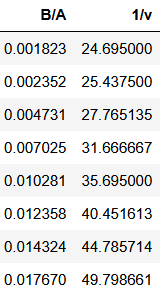
X7 = df2[["B/A"]]
y7 = df2["1/v"]

OLS7 = LinearRegression(fit_intercept=True).fit(X7, y7)

popt7 = solveOLS4(OLS7)
# array([4.78141520e-02, 7.65547585e+01])

df["xi7"] = model1(df["t"], *popt7)
score7 = metrics.r2_score(df["xi"], df["xi7"])
# 0.9996181966091182
Linearizations comparison
If we compare the four above linearization we get the following figure:
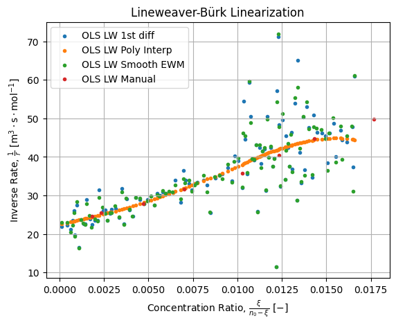
There are few things we can say on this figure above:
- All the points clouds exhibits the same trend;
- Crude and smoothed differences are noisy while polynomial difference is smooth put exhibits a pattern (notice it is a rational function in this plane);
- Manual estimation is not too bad for pre-numeric era technique;
Methods comparison
If we compare regressed constants by the different methods, we get the following table:
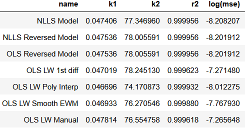
All methods return results in same order of magnitude and all score are at least 3 nines. Looking for the MSE we can confirm than minimum error is achieved by the reference which is expected.
If we draw them over the MSE landscape of the reference solution, we get the following figure:
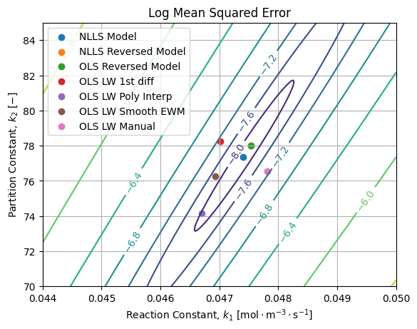
We can see the MSE landscape is at least locally convex close to the reference. Without surprise, best results are achieved by NLLS and OLS of the direct and reversed models. Because of the stretch of the error ellipsoid, it is possible to be closer to the reference with higher MSE (OLS LW 1st diff, OLS LW Manual) than results far away from reference with lower MSE (OLS LW Poly Interp, OLS LW Smooth EWM).
If we zoom out the MSE landscape, we get the following picture:
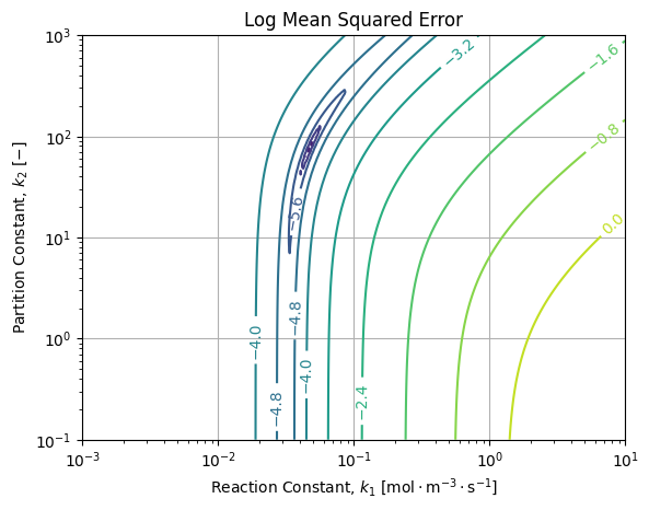
Which is non linear as expected and exhibits a single minimum for the given dataset and reference model over the field of plausible constant values. Therefore we may be confident the uniqueness of the solution and the stability of the reference algorithm.
Error structure
If we draw the distribution of absolute error wrt our reference model we get the following distribution:
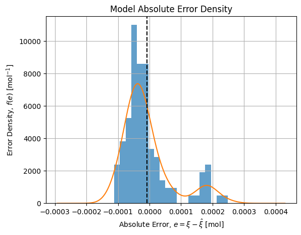
It shows a bimodal distribution that may be explained by a change of operator while manipulating:
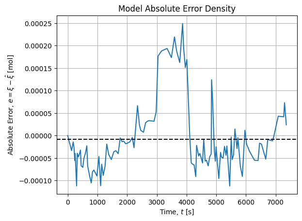
Between 2900 s and 4200 s, a switch of operator has been made, then the initial operator took over.
