Solving complex minimization problem

This post is a solution of the following question asked on Stack Overflow. It shows how to solve a complex minimization problem involving integral as objective function and differentials equations as constraints using the usual standard numpy and scipy libraries.

Problem Statement

The objective is to minimize the following quantity:

With respect to the following constraints:

Problem implementation

First we import the required libraries:

import functools
import numpy as np
import matplotlib.pyplot as plt
from scipy import integrate, optimize

We perform the problem discretization:

n = 121
t = np.linspace(0, 12, n)
dt = t[1] - t[0]

We guess some initial values:

x0 = np.array([
    0.5 * np.ones(shape=(n,)),
    0.7 * np.ones(shape=(n,)),
    np.zeros(shape=(n,)),
])

And define the bounds the solver must enforce:

bounds = np.array([
    [(0.5, 0.5)] + [(-np.inf, +np.inf)] * (n - 1),
    [(0.7, 0.7)] + [(-np.inf, +np.inf)] * (n - 1),
    [(0., 1.)] * n,
])

We then implement the objective function:

def integrand(x):
    x1, x2, v = x.reshape(3, -1)
    return (x1 - 1.) ** 2 + (x2 - 1.) ** 2

def integral(x, dt):
    return integrate.trapezoid(y=integrand(x), dx=dt)

The trick here is to reshape the x variable which is a flattened matrix of three variables.

Now we define the two non linear constraints:

def constraint1(x, dt):
    x1, x2, v = x.reshape(3, -1)
    return + x1 - x1 * x2 - 0.4 * x1 * v - np.gradient(x1, dt)

def constraint2(x, dt):
    x1, x2, v = x.reshape(3, -1)
    return - x2 + x1 * x2 - 0.2 * x2 * v - np.gradient(x2, dt)

At this point everything is setup to call the solver:

solution = optimize.minimize(
    method='SLSQP',
    fun=functools.partial(integral, dt=dt),
    x0=x0.ravel(),
    bounds=bounds.ravel().reshape(-1, 2),
    constraints=(
        optimize.NonlinearConstraint(functools.partial(constraint1, dt=dt), lb=0, ub=0),
        optimize.NonlinearConstraint(functools.partial(constraint2, dt=dt), lb=0, ub=0)
    ),
)

Where functions are parameterized with partial to cope with the extra dt parameter. The solution is about:

#      message: Optimization terminated successfully
#      success: True
#       status: 0
#          fun: 1.3444775334192278
#            x: [ 5.000e-01  5.036e-01 ...  4.060e-03  8.419e-04]
#          nit: 76
#          jac: [       nan -2.383e-02 ...  0.000e+00  0.000e+00]
#         nfev: 114155
#         njev: 76
#  multipliers: [ 7.009e-02  1.382e-01 ... -1.201e-05  6.489e-06]

We can estimate the integral value with respect to time:

It = integrand(solution.x).cumsum() * dt

Graphically the solution looks like:

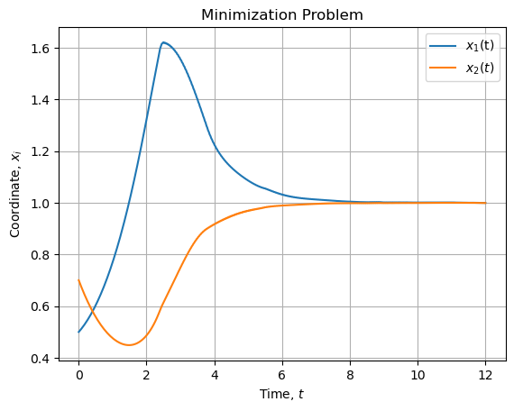
And the bounded coupling term looks like:

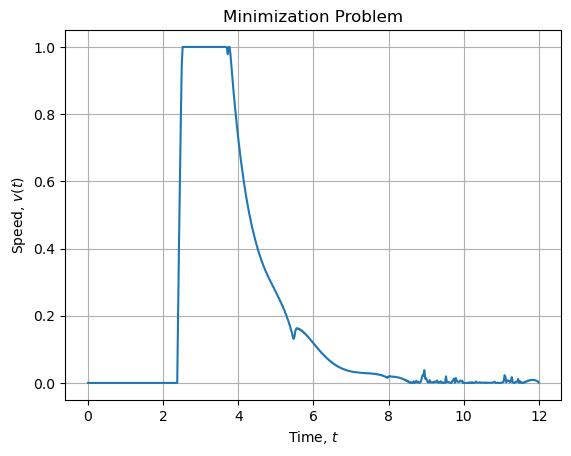
The phase portrait is about:

And the integral grows as follow with respect to time and coordinates: