The Lambert function is a less known function which has a lot nice applications in sciences.
The Lambert function is defined as follow:
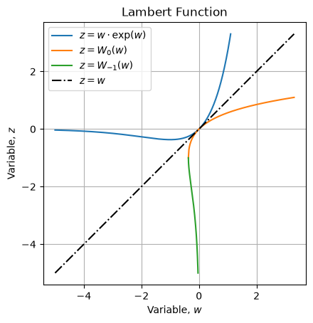
It is a multi-valued function with two real branches and . The figure below shows the real valued function and its inverses functions (real branches).
Michaelis-Menten
It can be shown that the Michaelis-Menten equation can lead to an analytical solution using the Lambert function. Given the Michaelis-Menten equation:
It is a separable ordinary differential equation, we can solve it explicitly for :
It goes as follow:
This is where the Lambert function comes into play, it allows us to isolate . First we rewrite the equation such as:
Then we simply apply the definition of the Lambert function:
Which is the analytical solution of the Michaelis-Menten equation.
Numerical solution
The Michaelis-Menten ODE can be solved numerically using Python and scipy for a given set of parameters and initial condition:
import numpy as np
from scipy import special, integrate, optimize
import matplotlib.pyplot as plt

K_M = 1e-3
v_max = 1e-4

def system(t, S, K_M, v_max):
    return np.array([
        - v_max * S[0] / (K_M + S[0])
    ])

t = np.linspace(0, 300, 200)
S0 = 1e-2

solution = integrate.solve_ivp(system, [t[0], t[-1]], [S0], t_eval=t, args=(K_M, v_max))
S = solution.y[0,:]
Now we can recover this parameters and initial condition by fitting the ODE solution using the analytical function found above:
def model(t, K_M, v_max, S_0):
    return np.real(K_M * special.lambertw((S_0 / K_M) * np.exp((- v_max * t + S_0) / K_M), 0))

popt, pcov = optimize.curve_fit(model, t, S)
Shat = model(t, *popt)
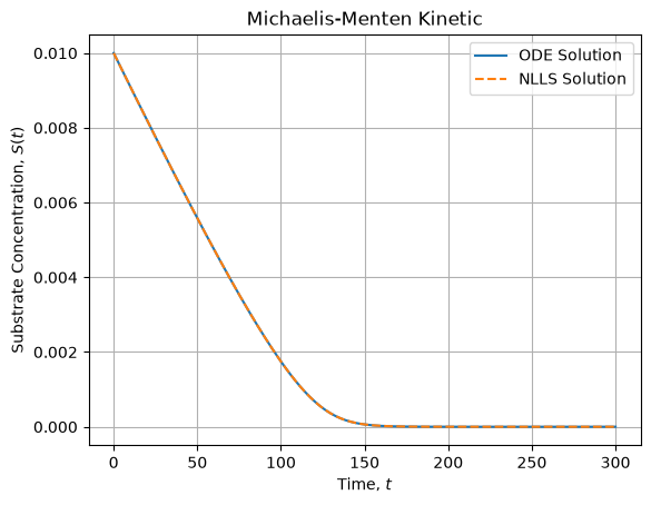
We can show that both model numerically agree:
Analytical solution
The Michaelis-Menten ODE can be solved analytically using Python and sympy package:
import sympy as sp

K = sp.Symbol("K", real=True, positive=True)
v = sp.Symbol("v", real=True, positive=True)
S0 = sp.Symbol("S0", real=True, positive=True)
t = sp.Symbol("t", real=True)
S = sp.Function("S")

equation = sp.Eq(sp.Derivative(S(t), t), - v * S(t) / (K + S(t)))

sp.dsolve(equation, ics={S(0): S0})
Which returns the above found function:
It can also be confirmed using Wolfram Alpha.