Logit Normal distribution

This post shows how to implement a missing distribution in scipy such as the Logit Normal distribution.

Definition

The logit function is defined as the inverse function of the expit function (or logistic function), such as:

A random variable $X$ is said to follow a Logit Normal distribution if and only if $Y = \mathrm{logit}(X)$ is normally distributed, conversely we may write $X = \mathrm{expit}(Y)$.

The density function of such a distribution is:

And looks like:

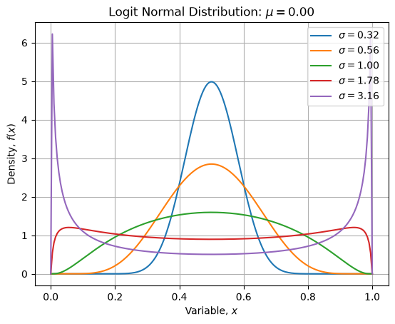
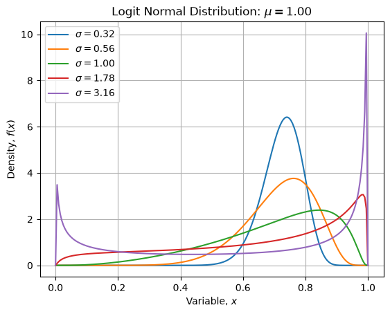
It can be symmetric or asymmetric, unimodal or bimodal based on the values of $\mu$ and $\sigma$. The distribution is quite versatile over its support $(0;1)$.

Implementation

The scipy package implements a lot of useful distributions using the class template stats.rv_continuous, but unfortunately not the Logit Normal distribution.

If we want to use the classic API for such a distribution, we must implement it by ourselves. To do so, we subclass the stats.rv_continuous class template and we must at least implement the _pdf (standing for Probability Density Function) or the _cdf (standing for Cumulative Density Function) function. It goes as follow:

from scipy import special, stats

class logitnorm_gen(stats.rv_continuous):

    def _argcheck(self, mu, sigma):
        return sigma > 0.
    
    def _pdf(self, x, mu, sigma):
        z = (special.logit(x) - mu) / sigma
        return stats.norm.pdf(z) / (sigma * x * (1. - x))
    
    def _cdf(self, x, mu, sigma):
        z = (special.logit(x) - mu) / sigma
        return stats.norm.cdf(z)

    def _ppf(self, q, mu, sigma):
        return special.expit(mu + sigma * stats.norm.ppf(q))

logitnorm = logitnorm_gen(a=0.0, b=1.0, name="logitnorm")

We have implemented both functions for performance sake in order to prevent numerical differentiation or integration each time it requires respectively the CDF or PDF.

For the same reason, we also have implemented the _ppf function in order to prevent numerical inversion the CDF each time it requires the quantile function (Percent-Point Function).

We also defined the support of the function and added a sanity check on the sigma parameter.

Usages

From there, we can use the logitnorm distribution in the same fashion than we can use the others scipy distributions without performance penalties.

Unitary area

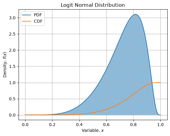
First we may assess that the PDF does have an unitary area:

from scipy import integrate

law = logitnorm(mu=1.12, sigma=0.76)
I, eps = integrate.quad(law.pdf, 0., 1.)
# (1.0000000000000078, 4.039395015138501e-10)

Which is true given the integration precision.

Sampling & fitting

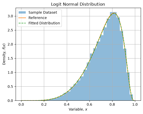
We can sample random dataset from the distribution and fit it against the model to estimate parameters:

sample = law.rvs(size=30_000, random_state=123456789)
popt = logitnorm.fit(sample, floc=0., fscale=1.)
# (1.1242027192507518, 0.7526448875694765, 0.0, 1.0)

Which is a fair Maximum Likelihood Estimation adjustment of the initial distribution.

Statistical Tests

We may perform statistical tests on our sampled dataset and adjusted distribution such as Kolmogorov Smirnov test:

fitted = logitnorm(*popt)
ks = stats.kstest(sample, fitted.cdf)
# KstestResult(statistic=0.0031606555408625336, pvalue=0.9244147334480032, ...)

Which is significant given the p-value of the test. We can also perform a Chi Squared test using equally probable bins to ensure enough bin counts for test purposes:

k = 10
bins = fitted.ppf(np.linspace(0., 1., k + 1))
obs = np.histogram(sample, bins=bins)[0]
ref = np.full(k, sample.size / k)
chi2 = stats.chisquare(obs, ref, ddof=2)
# Power_divergenceResult(statistic=4.023333333333333, pvalue=0.7770859730618183)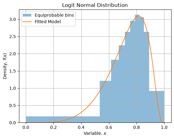

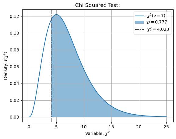
Which is significant given the p-value. We finally perform a Goodness of Fit test:

gof = stats.goodness_of_fit(logitnorm, sample, fit_params={"mu": popt[0], "sigma": popt[1], "loc": popt[2], "scale": popt[3]}, n_mc_samples=500)
# GoodnessOfFitResult(statistic=0.2364617410421488, pvalue=0.6327345309381237, ...)

Which is also significant given the p-value.

Testing

Finally we may automatize our tests to check it against various configurations:

def generate_fixtures(
    locs=[-2.0, -1.0, -0.5, 0.0, 0.5, 1.0, 2.0],
    scales=[0.32, 0.56, 1.00, 1.78, 3.16],
    sizes=[3_000, 30_000],
    seeds=[123, 456, 789, 123456, 123456789, 999999]
):
    for (loc, scale, size, seed) in itertools.product(locs, scales, sizes, seeds):
        yield {"parameters": {"loc": loc, "scale": scale}, "size": size, "random_state": seed}

for fixture in generate_fixtures():
    
    # Reference:
    parameters = fixture.pop("parameters")
    normal = stats.norm(**parameters)
    uniform = np.random.RandomState(fixture["random_state"]).uniform(size=fixture["size"])
    sample = special.expit(normal.ppf(uniform))
    
    # Logit Normal Law:
    law = logitnorm(mu=parameters["loc"], sigma=parameters["scale"])
    check = law.rvs(**fixture)
    
    # Fit:
    popt = logitnorm.fit(sample, floc=0.0, fscale=1.0)
    trial = logitnorm(*popt)

    # Tests:
    closeness = np.allclose(sample - check, 0.)   
    I, Ieps = integrate.quad(law.pdf, 0., 1.)
    ks = stats.kstest(check, trial.cdf)
    
    k = 10
    bins = trial.ppf(np.linspace(0., 1., k + 1))
    obs = np.histogram(sample, bins=bins)[0]
    ref = np.full(k, sample.size / k)
    chi2 = stats.chisquare(obs, ref, ddof=2)
    
    assert closeness
    assert np.allclose(I, 1., Ieps)
    assert ks.pvalue >= 0.005
    assert chi2.pvalue >= 0.005

For the given fixtures, all tests pass.

Conclusions

We have shown that its is possible to implement a missing scipy continuous variable distribution by subclassing the stats.rv_continuous class template.

We have at least implemented the _pdf function which is required to make the class works. We also have implemented the _cdf and _ppf functions for performances sake.

Then we have shown by simple examples the expected scipy API usage and performed some basic operations such as sampling, fitting and hypothesis testing.

Additionally, I have opened a feature request on the official GitHub scipy repository asking to add the above definition to the extensive long list of implemented distributions. Maybe in the future the Logit Normal distribution will be part of the package. Meanwhile the existing solution is still available if the missing distribution is needed.