Lastly I have recorded the Austen & Boelo Storms pressure variation with my bluebox – an indoor air quality measurement site embedding a BME-280 pressure sensor.
The story
I have build the bluebox in June 2021, the project embeds a Raspberry and sensors to monitor Temperature, Relative Humidity, Pressure (BME280), Carbon Dioxide (SCD30) and Particulate Matters (SPS30). The acquisition system is monitoring sensors over I2C with dedicated binary protocols to transduce them.
The BME280 already has recorded nice events such as the Hunga Tonga Volcano blast on 2021-01-15. This time, we will investigate a newer event related to atmospheric pressure: the Austen & Boelo Storms happening from 2026-10-23 to 2026-10-26.
Dataset
The raw dataset is sampled from 2026-10-17 09:00:00 to 2026-11-02 08:00:00 at Brussels (altitude 26.0m) with a time resolution of 10 seconds. This experimental dataset is then consolidated with a reference dataset of hourly meteorological data from the IRM-KMI public open data service (Uccle, altitude 101.3m).
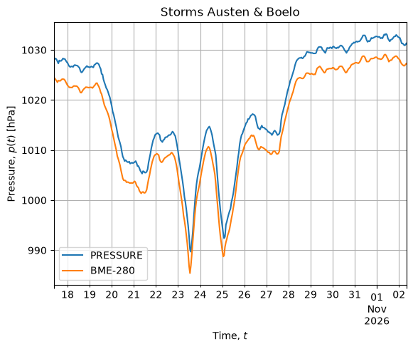
Both measurements show the exact same dynamic, the offset between the curves are explained mainly by the altitude difference. The Austen & Boelo Storms take place at the W shaped curves when the pressure drops significantly and suddenly, the first peak is Austen, the second is Boelo.
Sensor Calibration
If we compare the IRM Reference with our aggregated sensor, the calibration curve is as follow:
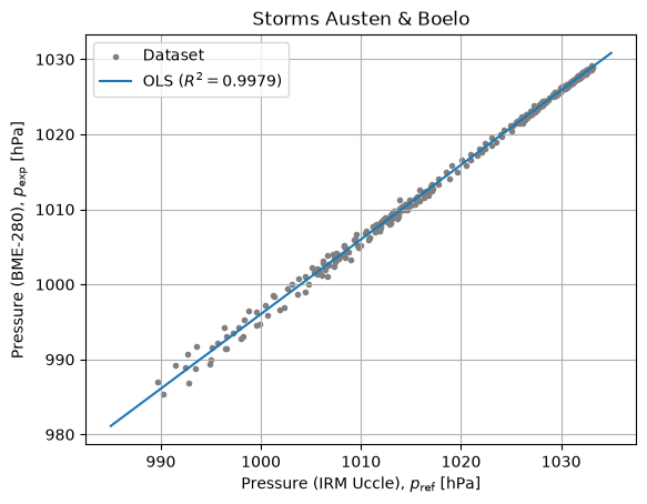
The calibration curve is with a coefficient of determination about 0.9979. Its slope is close to unity. The offset between the curves is then 4.0674 hPa which represents 33.8m of altitude difference. This pressure offset can be explained by the altitude difference and the pressure drop across the system (sensor is monitoring within a building so it is not directly exposed to the free atmosphere) and an intrinsic bias in the manufacturer calibration.
The figure below shows the error between both sensors:
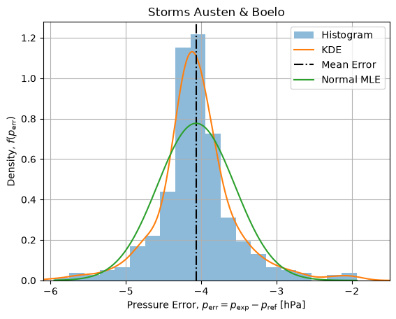
The error structure is quite symmetric but leptokurtic – it is sharper than a normal but has fatter tails, meaning that on the majority of recording are narrower than normal around the mean but outliers are stronger when occurring.
Wind Speed
Storms has strong pressure variations and also higher wind speed distributions.
The following figure shows the distribution of a year of hourly mean wind speed at IRM Uccle site:
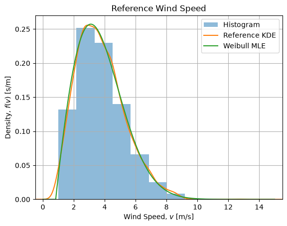
The MLE adjusted Weibull distribution nicely fits the histogram and the Kernel Density Estimation. A Kolmogorv-Smirnov test gives a statistic of 0.009949 and a p-value of 0.8195 which is significant.
Clustering
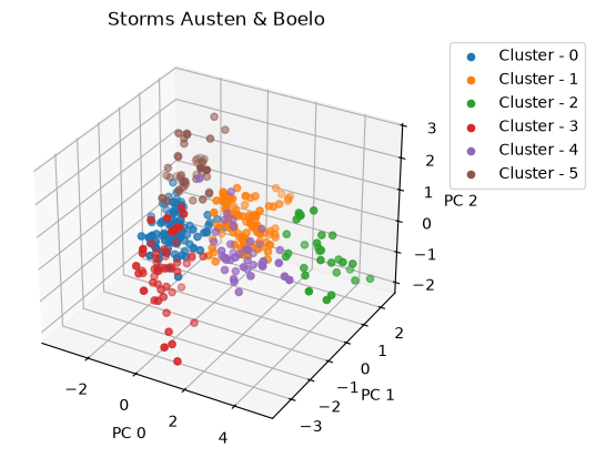
If we naively select the Storms peak, Wind Speed distributions contains artifacts and are mixed. We chose a different strategy, we selected 6 features: Pressure, Temperature, Relative Humidity, Wind Speed, Wind Direction and Wind Speed Peak. We standardize them and then we apply PCA to the dataset. Then we cluster the principal components by the mean of KMeans algorithm with 6 clusters.
The figure below shows the clusters over the three first principal components:
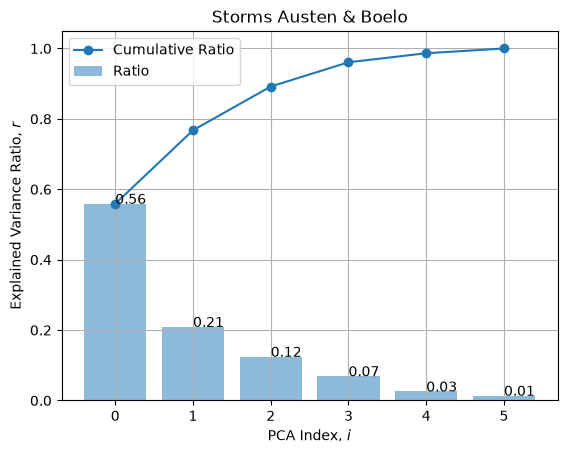
It can be shown that almost 90% of the sample variance can be captured by the three main components PC 0 – 2:
The PCA components are defined by the following matrix:
| PC 0 | PC 1 | PC 2 | PC 3 | PC 4 | PC 5 | |
|---|---|---|---|---|---|---|
| HUMIDITY_RELATIVE | -0.271244 | -0.488449 | 0.300747 | 0.321553 | 0.499525 | 0.494443 |
| PRESSURE | 0.670195 | -0.264928 | -0.620408 | 0.139900 | 0.196159 | 0.194151 |
| TEMP | -0.075307 | 0.040459 | -0.066351 | 0.913169 | -0.245514 | -0.306813 |
| WIND_DIRECTION | 0.661584 | -0.141126 | 0.710612 | 0.045116 | -0.179291 | -0.056920 |
| WIND_PEAK_SPEED | 0.169599 | 0.817370 | 0.101155 | 0.201285 | 0.308016 | 0.396889 |
| WIND_SPEED | 0.071671 | 0.039798 | 0.070996 | -0.024546 | 0.724362 | -0.680394 |
And loadings are about:
| PC 0 | PC 1 | PC 2 | PC 3 | PC 4 | PC 5 | |
|---|---|---|---|---|---|---|
| HUMIDITY_RELATIVE | -0.497267 | -0.547728 | 0.260028 | 0.207037 | 0.196026 | 0.140875 |
| PRESSURE | 1.228659 | -0.297080 | -0.536409 | 0.090077 | 0.076978 | 0.055317 |
| TEMP | -0.138059 | 0.045369 | -0.057367 | 0.587959 | -0.096346 | -0.087416 |
| WIND_DIRECTION | 1.212871 | -0.158253 | 0.614400 | 0.029049 | -0.070358 | -0.016218 |
| WIND_PEAK_SPEED | 0.310924 | 0.916566 | 0.087459 | 0.129601 | 0.120873 | 0.113080 |
| WIND_SPEED | 0.131393 | 0.044628 | 0.061384 | -0.015805 | 0.284259 | -0.193855 |
The figure below projects the Loadings on the two first principal components:
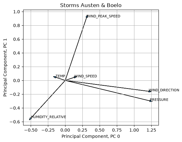
We can see that Pressure and Wind Direction strongly impacts the PC 0 in the same direction while they have mild effect on PC 1. Then Wind Speed Peak then strongly impacts PC 1 and mildly PC 0. Relative Humidity has mild impacts on both PC 0 and PC 1. Finally Wind Speed and Temperature has relatively small impacts on PC 0 and PC 1.
The figure below shows the clustered time series:
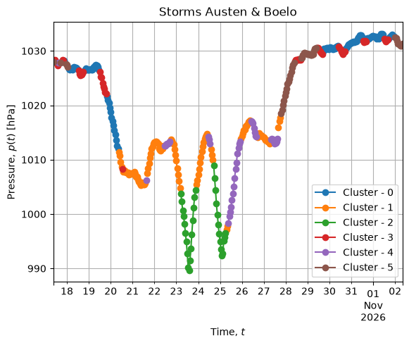
The Cluster – 2 is clearly the one containing the storm events. We can use it to assess the Wind Speed distribution of the storms to compare it with the reference distribution.
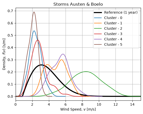
We can see that Cluster – 2 contains the Storms distribution, it is composed of higher wind speed than the reference distribution. Clusters – 1 and Cluster – 4 are storms context clusters while Cluster – 0, Cluster – 3 and Cluster – 5 are pre and post storms conditions.
Conclusions
We have shown that our BME-280 sensor is capable of following Atmospheric Pressure Variation accurately. The calibration curve has a slope close to unity and the pressure offset can be decomposed into three main effects: altitude difference, pressure drop through the system and intrinsic calibration bias.
We have shown that Reference Wind Speed distribution can be modeled as a Weibull distribution quite well for the selected reference sample (1 year).
We have clustered storm event using Standardized PCA and KMeans clustering. The PCA shows that loading are dominated by Pressure and Wind Direction which are the major impact variables, in the same fashion Wind Speed Peak and Relative Humidity are second order impact variables. While Temperature and Wind Speed are third order variables.